Download
1 / 21
210 likes | 421 Views
Design-plots for factorial and fractional-factorial designs. Russell R Barton Journal of Quality Technology ; 30, 1 ; Jan 1998 報告者:李秦漢. Outline. Introduction Hierarchical Frameworks for Design-Plots of Designs Fractional Designs, Graphical Projections and the Notion of Effect Sparsity

E N D
Design-plots for factorial and fractional-factorial designs Russell R Barton Journal of Quality Technology; 30, 1 ; Jan 1998 報告者:李秦漢
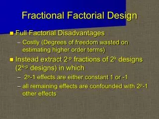
Outline • Introduction • Hierarchical Frameworks for Design-Plots of Designs • Fractional Designs, Graphical Projections and the Notion of Effect Sparsity • Graphical Patterns for confounding in Fractional-Factorial Designs • Presenting Experimental Results Using Response-Scaled Design-Plots
Introduction • This paper shows design-plots for fractional-factorial designs. • The primary focus of the paper is on two-level design. • The geometric properties of design-plots can be used to communicate design properties to non-statisticians. • A new plot, the response-scaled design-plot, allows a graphical interpretation of the experimental outcome using the design-plot framework.
Introduction • Response-scaled design-plots are used to display the results of the experiment, and in some cases this representation provides more insight than the values of the main-effect and interaction coefficients for the response model.
Hierarchical Frameworks for Design-Plots of Designs • Figure 1(a) shows a graphical representation for this simple two-run experiment. • Figure 1(b) shows a factorial experiment with two factors, A and B. • Figure 1(c) shows the runs for a factorial experiment. • The corner marked with an asterisk in Figure 1(c) corresponds to a run in which
Hierarchical Frameworks for Design-Plots of Designs • First level: The level of the hierarchy with a single instance of the design. • Inner design: If there are only two levels to the hierarchy, the first level will also be called the inner design. Ex: In Figure 1(d), the cube representation for factors A, B, C is the inner design; in figure 1(f) the square representation for factors C and D is the inner design.
Hierarchical Frameworks for Design-Plots of Designs • Figure 2 shows the framework for half-replicate designs with six and seven factors. • Figure 2(b) codes a seventh factor in the run symbol. An unfilled circle corresponds to a run with the seventh factor at its low value, and a filled circle represents a run with the seventh factor at its high value.
Fractional Designs, Graphical Projections and Notion of Effect Sparsity • A good design should provide significant coverage for all possible design projections. • Figure 3 shows two projections for a fractional design. The projection to the left is the result if factor D has no effect. The projection to the bottom is the result if factors C and E have no effect. (The inner square is projected to a line, and the outer cubes are projected to squares). In both cases the projected designs are full-factorials over the remaining factors. The CE projection gives two replicates at each point.
Fractional Designs, Graphical Projections and Notion of Effect Sparsity • Figure 4 shows a sequence of projections of the orthogonal array used by Taguchi and Wu (1980). • It is a fractional-factorial design, a subset of the design shown in Figure 2(b).
Graphical Patterns for confounding in Fractional-Factorial Designs A full-factorial experiment design model: The calculations for estimating the coefficient are illustrated in the left half of Figure 5.
Graphical Patterns for confounding in Fractional-Factorial Designs • Geometric patterns for the calculation of main effects and interactions for the design can be derived in a similar way. • The patterns for the design shown in Figure 6.
Graphical Patterns for confounding in Fractional-Factorial Designs • Direct confounding pattern: When run symbols occur at the locations corresponding to only one of the parity set (high or low) for a particular effect pattern, it is called a direct confounding pattern. Figure 7 shows run symbols only at the high value parity set for the ABC interaction. For direct confounding patterns, the observed design-plot pattern gives a word in the defining relation that corresponds to the effect estimated by that pattern. For Figure 7, the word is I=ABC.
Graphical Patterns for confounding in Fractional-Factorial Designs Figure 8 shows a hierarchical pattern for a design that generates I=ABC and I=DE. Consider augmenting the design in Figure 8 to be a design by adding the same small cube pattern to the large cube vertices for D high and E low, and D low and E high. In this case the large cube design would be a full factorial, so no word would be added. The defining relation would simply be I=ABC.
Graphical Patterns for confounding in Fractional-Factorial Designs On the other hand, if the parity set for the small cube pattern were changed at the uncircled large cube vertices, the pattern would match that of Figure 3. In this case the parity of the ABC pattern changes depending on the parity of the DE effect. The parity confounding pattern for the design in Figure 3 produces a word that is the concatenation of the large cube (DE) and small cube (ABC) patterns: I=ABCDE
Graphical Patterns for confounding in Fractional-Factorial Designs Figure 9 shows another design. The rear projection (removing factor B) shows an AC interaction pattern that changes parity with the value of E, creating the word I=ACE. The left projection removing factor D shows the same pattern. The lower projection shows and AB interaction pattern whose parity changes with D.The resulting defining relation for this design is I=ABD=ACE=BCDE.
Presenting Experimental Results Using Response-Scaled Design-Plots Response-scaled design-plots, scaling the size of each run symbol to correspond to the average magnitude of the response for the corresponding design factor settings. To achieve the best quantitative interpretation, areas of circles should be scaled by , with empirical studies giving values of . It is convenient to use , that is, the circle diameters are scaled proportionally to the average response. In some situations, response-scaled design-plots can provide more insight through direct observation than an examination of model coefficient estimates.
Presenting Experimental Results Using Response-Scaled Design-Plots Consider for example, a factorial experiment with nine replications per point. The results are listed in Table 1. Suppose that a higher response is preferable to a lower response in this case.
Presenting Experimental Results Using Response-Scaled Design-Plots Table 2 shows coefficient estimates based on these data for model: An ANOVA for the data in Table 1 shows all main effects, two-factor interactions, and the three-factor interaction are statistically significant.
Presenting Experimental Results Using Response-Scaled Design-Plots Interpretation of these results is difficult without a graphical presentation of the experimental outcomes. Figure 14 is the response-scaled design-plot for the data in Table 1. The plot makes the interpretation straight-forward. There is little difference among experimental conditions, except when all factors are at their high level. This information is not clear from the conventional model parameter estimates.
Presenting Experimental Results Using Response-Scaled Design-Plots Figure 15 shows the approach for a fraction of a design to estimate weld strength as a function of two design parameters (welding current and welding time) and three noise parameters (material thickness, air pressure, and surface cleanliness). A high weld strength is represented by a large circle, so setting the welding current to its high value and the welding time to its middle value produces the best result, that is, all of the circles on the cube at this location are large.
The End Thanks for your attention!