Download
1 / 19
190 likes | 287 Views
Computational Intelligence Winter Term 2010/11. Prof. Dr. Günter Rudolph Lehrstuhl für Algorithm Engineering (LS 11) Fakultät für Informatik TU Dortmund. Design of Evolutionary Algorithms. Three tasks: Choice of an appropriate problem representation.

E N D
ComputationalIntelligence Winter Term 2010/11 Prof. Dr. Günter Rudolph Lehrstuhl für Algorithm Engineering (LS 11) Fakultät für Informatik TU Dortmund
Design of Evolutionary Algorithms • Three tasks: • Choice of an appropriate problem representation. • Choice / design of variation operators acting in problem representation. • Choice of strategy parameters (includes initialization). ad 1) different “schools“: (a) operate on binary representation and define genotype/phenotype mapping+ can use standard algorithm– mapping may induce unintentional bias in search (b) no doctrine: use “most natural” representation – must design variation operators for specific representation+ if design done properly then no bias in search G. Rudolph: ComputationalIntelligence▪ Winter Term 2010/11 2
Design of Evolutionary Algorithms ad 2)design guidelines for variation operators • reachabilityevery x 2 X should be reachable from arbitrary x02 Xafter finite number of repeated variations with positive probability bounded from 0 • unbiasednessunless having gathered knowledge about problemvariation operator should not favor particular subsets of solutions) formally: maximum entropy principle • controlvariation operator should have parameters affecting shape of distributions;known from theory: weaken variation strength when approaching optimum G. Rudolph: ComputationalIntelligence▪ Winter Term 2010/11 3
Design of Evolutionary Algorithms ad 2)design guidelines for variation operators in practice binary search space X = Bn variation by k-point or uniform crossover and subsequent mutation a) reachability: regardless of the output of crossover we can move from x 2Bn to y 2Bn in 1 step with probability where H(x,y) is Hamming distance between x and y. Since min{ p(x,y): x,y 2Bn } = > 0 we are done. G. Rudolph: ComputationalIntelligence▪ Winter Term 2010/11 4
Design of Evolutionary Algorithms b) unbiasedness don‘t prefer any direction or subset of points without reason ) use maximum entropy distribution for sampling! • properties: • distributes probability mass as uniform as possible • additional knowledge can be included as constraints:→ under given constraints sample as uniform as possible G. Rudolph: ComputationalIntelligence▪ Winter Term 2010/11 5
Design of Evolutionary Algorithms Formally: Definition: Let X bediscreterandom variable (r.v.) withpk = P{ X = xk } forsomeindexset K.The quantity iscalledtheentropyofthedistributionof X. If X is a continuousr.v. withp.d.f. fX(¢) thentheentropyisgivenby The distributionof a random variable X forwhich H(X) is maximal istermed a maximumentropydistribution. ■ G. Rudolph: ComputationalIntelligence▪ Winter Term 2010/11 6
s.t. solution: via Lagrange (find stationary point of Lagrangian function) Excursion: Maximum Entropy Distributions Knowledge available: Discrete distribution with support { x1, x2, … xn } with x1 < x2 < … xn < 1 ) leadstononlinearconstrainedoptimizationproblem: G. Rudolph: ComputationalIntelligence▪ Winter Term 2010/11 7
partial derivatives: ) uniform distribution ) Excursion: Maximum Entropy Distributions G. Rudolph: ComputationalIntelligence▪ Winter Term 2010/11 8
) leadstononlinearconstrainedoptimizationproblem: s.t. and solution: via Lagrange (find stationary point of Lagrangian function) Excursion: Maximum Entropy Distributions Knowledge available: Discrete distribution with support { 1, 2, …, n } with pk = P { X = k } and E[ X ] = G. Rudolph: ComputationalIntelligence▪ Winter Term 2010/11 9
* ( ) Excursion: Maximum Entropy Distributions partial derivatives: ) ) (continued on next slide) G. Rudolph: ComputationalIntelligence▪ Winter Term 2010/11 10
) ) discrete Boltzmann distribution ) value of q depends on via third condition: * ( ) Excursion: Maximum Entropy Distributions ) G. Rudolph: ComputationalIntelligence▪ Winter Term 2010/11 11
Excursion: Maximum Entropy Distributions = 8 = 2 Boltzmann distribution (n = 9) = 7 specializes to uniform distribution if = 5 (as expected) = 3 = 5 = 6 = 4 G. Rudolph: ComputationalIntelligence▪ Winter Term 2010/11 12
solution: in principle, via Lagrange (find stationary point of Lagrangian function) but very complicated analytically, if possible at all ) consider special cases only Excursion: Maximum Entropy Distributions Knowledge available: Discrete distribution with support { 1, 2, …, n } with E[ X ] = and V[ X ] = 2 ) leadstononlinearconstrainedoptimizationproblem: and and s.t. note: constraints are linear equations in pk G. Rudolph: ComputationalIntelligence▪ Winter Term 2010/11 13
Linear constraints uniquely determine distribution: I. II. III. II – I: I – III: unimodal uniform bimodal Excursion: Maximum Entropy Distributions Special case: n = 3andE[ X ] = 2 and V[ X ] = 2 insertion in III. G. Rudolph: ComputationalIntelligence▪ Winter Term 2010/11 14
solution: via Lagrange (find stationary point of Lagrangian function) Excursion: Maximum Entropy Distributions Knowledge available: Discrete distribution with unbounded support { 0, 1, 2, … } and E[ X ] = ) leads to infinite-dimensional nonlinear constrained optimization problem: s.t. and G. Rudolph: ComputationalIntelligence▪ Winter Term 2010/11 15
partial derivatives: ) * ( ) Excursion: Maximum Entropy Distributions ) (continued on next slide) G. Rudolph: ComputationalIntelligence▪ Winter Term 2010/11 16
insert ) set and insists that ) for geometrical distribution it remains to specify q; to proceed recall that Excursion: Maximum Entropy Distributions ) ) G. Rudolph: ComputationalIntelligence▪ Winter Term 2010/11 17
) * ( ) Excursion: Maximum Entropy Distributions ) value of q depends on via third condition: ) G. Rudolph: ComputationalIntelligence▪ Winter Term 2010/11 18
Excursion: Maximum Entropy Distributions = 1 = 7 geometrical distribution with E[ x ] = = 2 = 6 pk only shown for k = 0, 1, …, 8 = 3 = 4 = 5 G. Rudolph: ComputationalIntelligence▪ Winter Term 2010/11 19