Download
1 / 54
540 likes | 543 Views
Explore the typical distribution patterns of water properties such as temperature, salinity, density, and other tracers. Learn about ventilation, isopycnals, water masses, and more.

E N D
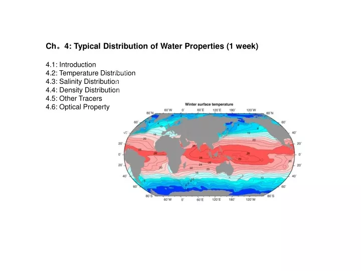
Ch。4: Typical Distribution of Water Properties (1week) 4.1: Introduction 4.2: Temperature Distribution 4.3: Salinity Distribution 4.4: Density Distribution 4.5: Other Tracers 4.6: Optical Property Features: ranges from -1.8oC to 30oC Features: ranges from -1.8oC to 30oC
4.1: Introduction Surface temperature from -1.8oC to 30oC Features: ranges from -1.8oC to 30oC Q: where will be the bottom water originating from ?
Basic concepts Ventilation: connection of water property from the surface to the interior Isopycnal: along isopycnal surfaces Water Mass: caused by an identifiable single source (of relatively uniform property) The sea waters are limited to a small range of T-S, 75%, 0-6C, 34-35 ppt 50%, 1.3-3.8C, 34.6-34.8 ppt mean, 3.5C, 34.7 ppt Ventilation through localized convection Potential Temperature Salinity Ventilation along isopycanls North Atlantic Deep Water Sigma_t, Sigma_4 Dissolved Oxygen
4.2: Temperature (a) Surface temperature (°C) of the oceans in winter (January, February, March north of the equator; July, August, September south of the equator) based on averaged (climatological) data from Levitus and Boyer (1994). (b) Satellite infrared sea surface temperature (°C; nighttime only), averaged to 50 km and 1 week, for January 3, 2008. White is sea ice. Source:From NOAA NESDIS (2009). Surface Temperature Distribution quasi-zonal, why ? solar radiation (y), atmosphere effect such as wind, colder equator (in the eastern part), why ? upwelling and ocean dynamics, important to ENSO, East/West asymmetry in the midlatitude: West warm/ East cold, why ? gyre circulation, western boundary currents, North /South asymmetry, cold tongue from the southern hemisphere, why ? geometry ocean-atmosphere coupling (also, annual cycle) FIGURE 4.1
Variation with latitude of surface (a) temperature, (b) salinity, and (c) density averaged for all oceans for winter. North of the equator: January, February, and March. South of the equator: July, August, and September. Based on averaged (climatological) data from Levitus and Boyer (1994) and Levitus et al. (1994b). Surface Temperature, Salinity, and Density Temperature Salinity Sigma_t FIGURE 4.3
Last Glacial Maximum (21,000 years ago) CLIMAP Reconstruction Colder ! LGM August SST LGM- present August SST
Typical potential temperature (°C)/depth (m) profiles for the open ocean in (a) the tropical western North Pacific (5°N), (b) the western and eastern subtropical North Pacific (24°N), and (c) the western subpolar North Pacific (47°N). Corresponding salinity profiles are shown in Figure 4.16. Vertical Temperature Distribution Mixed layer: ~1-m (summer, low lat) <--> ~1000-m (winter, high lat localized deep convection region) (seasonal thermocline) Thermocline: sharp gradient below mixed layer to abyssal layers (permanent thermocline) Abyssal layers: intermediate water, deep water and bottom water FIGURE 4.2
Mixed layer depth in (a) January and (b) July, based on a temperature difference of 0.2°C from the near-surface temperature. (c) Averaged maximum mixed layer depth, using the 5 deepest mixed layers in 1° ´ 1° bins from the Argo profiling float data set (2000-2009). Mixed layer depth Wind stirring can lead to mixed layer depth of ~ 100-m in winter (over a broad region!) Surface buoyance flux (cooling or evaporation), on the other hand, can generate isolated deep convection of ~1000-m Maximum mixed layer depth (late winter) is the depth surface water property (temp, salinity, co2, …) leaks (or subducts) into the permanent thermocline (why? Stommel’s Demon) FIGURE 4.4
Mixed layer development. (a, b) An initially stratified layer mixed by turbulence created by wind stress; (c, d, e) an initial mixed layer subjected to heat loss at the surface which deepens the mixed layer; (f, g, h) an initial mixed layer subjected to heat gain and then to turbulent mixing presumably by the wind, resulting in a thinner mixed layer; (i, j) an initially stratified profile subjected to internal mixing, which creates a stepped profile. Notation: t is wind stress, Q is heat (buoyancy). Formation mechanism of mixed layer FIGURE 7.3
Growth and decay of the seasonal thermocline at 50°N, 145°W in the eastern North Pacific (Ocean Station P (Papa)) as (a) vertical temperature profiles, (b) time series of isothermal contours, and (c) a time series of temperatures at depths shown. Seasonal Mixed layer/Seasonal Thermocline Maximum mixed layer depth (late winter) is the depth surface water property (temp, salinity, co2, …) leaks (or subducts) into the permanent thermocline, while waters at shallower depth will be taken by the mixing of the next winter before subducting into the permanent thermocline Stommel’s Demon FIGURE 4.8
Amplitude of SST Seasonal Cycle Annual range of sea surface temperature (°C), based on monthly climatological temperatures from the World Ocean Atlas (WOA05) (NODC, 2005a, 2009). Why minimum? Why maximum? Why minimum? • Amplitude of seasonal cycle in the subsurface temperature? almost 0 below 2-300 m • Diurnal cycle ? up to 1-3oC to depth of up to 1-m, strong in low wind, high insolation region (subtropics..) FIGURE 4.9
Thermocline (permanent thermocline, main thermocline) How to maintain a sharp gradient? Potential Temperature Salinity North Atlantic Deep Water Sigma_t, Sigma_4 Dissolved Oxygen FIGURE 4.5
1-D advective-diffusive thermocline: Cold upwelling balancing downward heat flux wTz = A (Tz)z Thermocline thickness h ~ A/w ~ 1 cm^2/s / 10^(-4)cm/s ~100 m heat flux ATz buoyancy driven cold upwelling wT , w~ 1 cm/day Equator North Advective-Diffusive Thermocline 1-D Model: Advective-Diffusive Thermocline h FIGURE 4.5
Temperature-salinity along surface swaths in the North Atlantic (dots and squares), and in the vertical (solid curves) at stations in the western North Atlantic (Sargasso Sea) and eastern North Atlantic. Source: From Iselin (1939). Subduction and Ventilated Thermocline (subtropics) Subduction/ventilation FIGURE 4.6
Advective Thermocline (ventilated) heat flux Ekman pumping warm downwelling wT wind driven cold advection vT 2-D Model: Advective Thermocline 2-D advective thermocline (subtropics only!) Warm downwelling balanced by cold advection vTy + wTz = 0 thermocline thickness h ~ sqrt( tau*L/rho*g’) ~ sqrt (1dyn/cm^2 * 10^8 cm /1g/cm^3/1s^2) ~ 100 m h FIGURE 4.5
Potential temperature-salinity relation in the thermocline of each subtropical gyre. These are the Central Waters. R is the best fit of a parameter associated with double diffusive mixing (Section 7.4.3). Source: From Schmitt (1981). Central Waters (masses) freshest Saltiest FIGURE 4.7
Double Thermocline, Mode Water The two mechanisms of thermocline can be mixed, and usually advective is in the upper part and diffusive is in the lower part. In the subtropical western side, the two thermocline show a clear separation by a mode water (thermostad) Advective thermocline: upper thermocline Diffusive Thermocline: lower thermocline FIGURE 4.2
Subduction/ventilation Advective thermocline: upper thermocline Thermostad (Mode Water) Diffusive Thermocline: lower thermocline Potential Temperature Salinity Advective thermocline: upper thermocline Diffusive Thermocline: lower thermocline Mode Water North Atlantic Deep Water Sigma_t, Sigma_4 Dissolved Oxygen
Deep Water Temperature, Potential Temperature, Mariana Trench: (a) in situ temperature, T, and potential temperature, q (°C); (b) salinity (psu); (c) potential density sq (kg m–3) relative to the sea surface; and (d) potential density s10 (kg m–3) relative to 10,000 dbar. FIGURE 4.10
Vertical Temperature Distribution (a) Potential temperature (°C), (b) salinity (psu), (c) potential density sq (top) and potential density s4 (bottom) (kg m–3), and (d) oxygen (mmol/kg) in the Atlantic Ocean at longitude 20° to 25°W. Data from the World Ocean Circulation Experiment. Atlantic Ocean FIGURE 4.11
Pacific Ocean (a) Potential temperature (°C), (b) salinity (psu), (c) potential density sq (top) and potential density s4 (bottom; kg m–3), and (d) oxygen (mmol/kg) in the Pacific Ocean at longitude 150°W. Data from the World Ocean Circulation Experiment. FIGURE 4.12
(a) Potential temperature (°C), (b) salinity (psu), (c) potential density sq (top) and potential density s4 (bottom; kgm–3), and (d) oxygen (mmol/kg) in the Indian Ocean at longitude 95°E. Data from the World Ocean Circulation Experiment. Indian Ocean FIGURE 4.13
4.3: Salinity Distribution Mean salinity, zonally averaged and from top to bottom, based on hydrographic section data. The overall mean salinity is for just these sections and does not include the Arctic, Southern Ocean, or marginal seas. Column Average S Most salty Most fresh FIGURE 4.14
Sea Surface Salinity Surface salinity (psu) in winter (January, February, and March north of the equator; July, August, and September south of the equator) based on averaged (climatological) data from Levitus et al. (1994b). Q: Why Salty N. Atlantic and fresh N. Pacific? SSS 39 41 E-P Net evaporation and precipitation (E–P) (cm/yr) based on climatological annual mean data(1979–2005) from the National Center for Environmental Prediction. Net precipitation is negative (blue), net evaporation is positive (red). Overlain: freshwater transport divergences (Sverdrups or 1×10⁹ kg/sec) based on ocean velocity and salinity observations. FIGURE 4.15, 5.4a
Pacific Atlantic ascend sink deep branch surface branch Convelt Belt Why Salty N. Atlantic and fresh N. Pacific? A positive feedback, for self sustaining Positive feedback Triggers ? NA higher lat, narrow width Pacific, Tibet and Asian monsoon ……??
North Pacific. Vertical Salinity Profiles Salinity Temperature FIGURE 4.16
Vertical Salinity Distribution and Water Masses Much more complicated than temperature, more like tracer for water masses (a) Potential temperature (°C), (b) salinity (psu), (c) potential density sq (top) and potential density s4 (bottom) (kg m–3), and (d) oxygen (mmol/kg) in the Atlantic Ocean at longitude 20° to 25°W. Data from the World Ocean Circulation Experiment. Atlantic Ocean Subtropical underwater (salinity maximum water, central water) Antarctic Intermediate Water (AAIW, fresh) Antarctic Bottom Water (AABW) (cold and fresh) Subarctic Intermediate Water (shallow salinity minimum) Labrado Sea Water (LSW) Mediterreanina source North Atlantic Deep Water (NADW, salty relative to deep Antarctic) FIGURE 4.11
Pacific Ocean Subtropical underwater (salinity maximum water, central water) AAIW North Pacific Intermediate Water (shallow salinity minimum) Pacific Deep Water NADW (a) Potential temperature (°C), (b) salinity (psu), (c) potential density sq (top) and potential density s4 (bottom; kg m–3), and (d) oxygen (mmol/kg) in the Pacific Ocean at longitude 150°W. Data from the World Ocean Circulation Experiment. FIGURE 4.12
(a) Potential temperature (°C), (b) salinity (psu), (c) potential density sq (top) and potential density s4 (bottom; kgm–3), and (d) oxygen (mmol/kg) in the Indian Ocean at longitude 95°E. Data from the World Ocean Circulation Experiment. Indian Ocean Red Sea source Subtropical underwater AAIW NADW AABW Indian Ocean Deep Water FIGURE 4.13
North Pacific. Vertical Salinity Profiles Subtroical underwater NPIW Salinity NADW Temperature FIGURE 4.16
Deep Water Temperature and Salinity Deep and bottom waters. (a) Distribution of waters that are denser than s4 = 45.92 kg/m3. This is approximately the shallowest isopycnal along which the Nordic Seas dense waters are physically separated from the Antarctic’s dense waters. At lower densities, both sources are active, but the waters are intermingled. Large dots indicate the primary formation site of each water mass; fainter dots mark the straits connecting the Nordic Seas to the open ocean. The approximate potential density of formation is listed. Source: After Talley (1999). (b) Potential temperature (°C), and (c) salinity at the ocean bottom, for depths greater than 3500 m. FIGURE 14.14bc
T-S-Volume Potential temperature-salinity-volume (q-S-V) diagrams for (a) the whole water column and (b) for waters colder than 4°C. The shaded region in (a) corresponds to the figure in (b). Source: From Worthington (1981). FIGURE 4.17
4.4: Density Distribution Surface density sq (kg m–3) in winter (January, February, and March north of the equator; July, August, and September south of the equator) based on averaged (climatological) data from Levitus and Boyer (1994) and Levitus et al. (1994b). horizontal variation 2-4 0/00 << 40 0/00 vertical variation FIGURE 4.19
Potential Density Distribution (a) Potential density sq (kg m–3) and (b) neutral density gN in the Atlantic Ocean at longitude 20° to 25°W. Compare with Figure 4.12c. Data from the World Ocean Circulation Experiment. horizontal variation 2-4 0/00 ~ vertical variation Unstable? FIGURE 4.18
Vertical Profile of Density and Potential Density Thermocline in T pycnocline in density Typical density/depth profiles for low and high latitudes (North Pacific). Pycnocline FIGURE 4.20
(a) Potential temperature (°C), (b) salinity (psu), (c) potential density sq (top) and potential density s4 (bottom) (kg m–3), and (d) oxygen (mmol/kg) in the Atlantic Ocean at longitude 20° to 25°W. Data from the World Ocean Circulation Experiment. Vertical Density Distribution: Mostly similar to temperature except for high latitude Atlantic Ocean FIGURE 4.11
Pacific Ocean (a) Potential temperature (°C), (b) salinity (psu), (c) potential density sq (top) and potential density s4 (bottom; kg m–3), and (d) oxygen (mmol/kg) in the Pacific Ocean at longitude 150°W. Data from the World Ocean Circulation Experiment. FIGURE 4.12
(a) Potential temperature (°C), (b) salinity (psu), (c) potential density sq (top) and potential density s4 (bottom; kgm–3), and (d) oxygen (mmol/kg) in the Indian Ocean at longitude 95°E. Data from the World Ocean Circulation Experiment. Indian Ocean FIGURE 4.13
4.5: Other Tracers Dissolved Oxygen O2 Source: generated at surface with air-sea exchange, usually saturation 100%, with some enhancement by photosynthesis (oversaturation) Sink: consumed by living organism and bacteria oxidation so an indication of ventilation age Nutrients (Silica, Nitrate, Phosphate, Nitrite…) Sink: utilization by phytoplantkton in the surface layer (euphotic zone, exposed to sunlight) Source: increase in deep waters because of their release back to solution by biological processes (respiration, nitrification) during the decay of detrital material sinking from the upper ocean So, approximately a mirror image of oxygen! Age Tracers (CFC12/13, tritium, D14C…) Source: surface air-sea exchange Sink: naturally decaying with half life time of ~10 -- 10000 years The importance of tracer in ocean study: Direct measurements of interior flow (<1 cm/s) is very difficult, tracer provides a powerful way of estimating the water circulation. (This is different from atmosphere, in which direct measurements of winds are easy). However, it should be noticed that the inversion of tracer to velocity field is very complicated. So, in interpreting the ocean circulation from tracer distribution, one should be cautious. Having various sets of tracers consistent is important.
Vertical Dissolved Oxygen Distribution: More similar to salinity as a tracer, Moreover, a tracer for ventilation time (but non-conservative because of biological activity!) (a) Potential temperature (°C), (b) salinity (psu), (c) potential density sq (top) and potential density s4 (bottom) (kg m–3), and (d) oxygen (mmol/kg) in the Atlantic Ocean at longitude 20° to 25°W. Data from the World Ocean Circulation Experiment. Dissolved oxygen: Source: generated at surface with air-sea exchange, usually saturation 100%, with some enhancement by photosynthesis (oversaturation) Sink: consumed by living organism and bacteria oxidation so an indication of ventilation age Atlantic Ocean Oxygen Minimum Zone 1.Minimum circulation 2.Increased density accumulates detritus, increasing oxidation rate 3.Bottom water fresher through convection ventilation from the Atlantic FIGURE 4.11
Pacific Ocean (a) Potential temperature (°C), (b) salinity (psu), (c) potential density sq (top) and potential density s4 (bottom; kg m–3), and (d) oxygen (mmol/kg) in the Pacific Ocean at longitude 150°W. Data from the World Ocean Circulation Experiment. OMZ FIGURE 4.12
(a) Potential temperature (°C), (b) salinity (psu), (c) potential density sq (top) and potential density s4 (bottom; kgm–3), and (d) oxygen (mmol/kg) in the Indian Ocean at longitude 95°E. Data from the World Ocean Circulation Experiment. Indian Ocean OMZ FIGURE 4.13
Profiles of dissolved oxygen (mmol/kg) from the Atlantic (gray) and Pacific (black) Oceans. (a) 45°S, (b) 10°N, (c) 47°N. Vertical Dissolved Oxygen Distribution Pacific vs Atlantic OMZ: N. Pacific lower than N. Atlantic FIGURE 4.21
Nitrate (mmol/kg) and dissolved silica (mmol/kg) for the Atlantic Ocean (a, b), the Pacific Ocean (c, d), and the Indian Ocean (e, f). Note that the horizontal axes for each ocean differ. Vertical Nutrient Distribution Nitrate Dissolved silica Dissolved Oxygen Atlantic Ocean Pacific Ocean Indian Ocean FIGURE 4.22
Nitrate (mmol/L) at the sea surface, from the climatological data set of Conkright, Levitus, and Boyer (1994). FIGURE 4.23
(a) Chlorofluorocarbon content (CFC-11; pmol/kg) and (b) D14C (/mille) in the Pacific Ocean at150°W. White areas in (a) indicate undetectable CFC-11. Age Tracers Age tracer concentration and water age C(t)=C0exp(-t/T) C0: C value at the surface C(t): in situ concentration Age: time away from the surface Age=t=-tao*ln(C(t)/C0) Half time T ~ 10 years for CFC 5600 years for D14C CFC-11 (anthropogenic source) t~ decades ~0 D14C (cosmic ray) t~ 500-1000 years Pacific Ocean 250 years Atlantic Ocean 250 years Indian Ocean FIGURE 4.24
(a) Age (years) of Pacific Ocean waters on the isopycnal surface 27.2 sq, using the ratio of chlorofluorocarbon-11 to chlorofluorocarbon-12.. (b) Tritium concentration at 500 m in the Pacific Ocean from the WOCE Pacific Ocean Atlas. Tritium (half time 12 years, 3H=>3He CFC-11/12 FIGURE 4.25
Age Tracers If the water is contributed by a single source, the age estimation is straightforward using the decaying time. In general, a tracer is contributed by multiple sources at the surface from different regions. This makes the estimation of water age complicated. One can show that the decay age is usually biased towards the youngest water. That is the real water age is older than the decaying age because of the mixing with older waters. Ref. Siberlin C. and C. Wunsch, 2011: Oceanic tracer and proxy time scales revisited. Clim. Past, 7, 27-39. Primeau F. and E. Deleersnijder, 2009: On the time to tracer equilibrium in the global ocean. Ocean Science, 5, 13-28. Also, surface air-sea interaction and sea ice will also affect the age at the surface (or the reservoir age). Ventilation rate (production rate) is the rate of new water injection into a reservoir Vrate= Volume/age Turnover time is the time it takes to replenish a reservoir Tturnover = V/Rout = Volume/Export Flux Residence Time is the time a particle spends within a reservoir.
Mean Secchi disk depths as functions of latitude in the Pacific and Atlantic Oceans. Old instrument: Secchi disk Reduced depth and increased ch-a, due to more organic matters associated with upwelling of nutrients which feeds biological activities. Traditional method of visual exminenation of the depth of a painted disk (SECCHI disk). The deeper the cleaner, the deeper penetration, the less organic material and less cholrophyll-a (green pigment). FIGURE 4.26