Download
1 / 48
510 likes | 668 Views
Unsupervised learning The Hebb rule – Neurons that fire together wire together. PCA RF development with PCA. Classical Conditioning and Hebb’s rule. Ear. A. Nose. B. Tongue. “When an axon in cell A is near enough to excite cell B and

E N D
Unsupervised learning • The Hebb rule – Neurons that fire together wire together. • PCA • RF development with PCA
Classical Conditioning and Hebb’s rule Ear A Nose B Tongue “When an axon in cell A is near enough to excite cell B and repeatedly and persistently takes part in firing it, some growth process or metabolic change takes place in one or both cells such that A’s efficacy in firing B is increased” D. O. Hebb (1949)
The generalized Hebb rule: where xiare the inputs and y the output is assumed linear: Results in 2D
Example of Hebb in 2D w (Note: here inputs have a mean of zero)
On the board: • Solve simple linear first order ODE • Fixed points and their stability for non linear ODE.
In the simplest case, the change in synaptic weight w is: where xare input vectors and y is the neural response. Assume for simplicity a linear neuron: So we get: Now take an average with respect to the distribution of inputs, get:
If a small change Δw occurs over a short time Δt then: (in matrix notation) If <x>=0 , Q is the covariance function. What is then the solution of this simple first order linear ODE ? (Show on board)
Mathematics of the generalized Hebb rule The change in synaptic weight w is: where x are input vectors and y is the neural response. Assume for simplicity a linear neuron: So we get:
Taking an average of the the distribution of inputs And using and We obtain
In matrix form Where J is a matrix of ones, e is a unit vector in direction (1,1,1 … 1), and or Where
The equation therefore has the form If k1 is not zero, this has a fixed point, however it is usually not stable. If k1=0 then have:
The Hebb rule is unstable – how can it be stabilized while preserving its properties? The stabilized Hebb (Oja) rule. Normalize Where |w(t)|=1 Appoximate to first order in Δw: (show on board) Now insert Get:
} y Therefore The Oja rule therefore has the form:
Average In matrix form:
Using this rule the weight vector converges to • the eigen-vector of Q with the highest eigen-value. It is often called a principal component or PCA rule. • The exact dynamics of the Oja rule have been solved by Wyatt and Elfaldel 1995 • Variants of networks that extract several principal components have been proposed (e.g: Sanger 1989)
Therefore a stabilized Hebb (Oja neuron) carries out Eigen-vector, or principal component analysis (PCA).
Using this rule the weight vector converges to the eigen-vector of Q with the highest eigen-value. It is often called a principal component or PCA rule. Another way to look at this: Where for the Oja rule: At the f.p: where So the f.p is an eigen-vector of Q. The condition means that w is normalized. Why? Could there be other choices for β?
Show that the Oja rule converges to the state |w^2|=1 The Oja rule in matrix form: What is Bonus question for H.W: The equivalence above, why does it prove convergence to normalization.
Show that the f.p of the Oja rule is such that the largest eigen-vector with the largest eigen-value (PC) is stable while others are not (from HKP – pg 202). Start with: Assume w=ua+εub where ua and ub are eigen-vectors with eigen-values λa,b
Get: (show on board) Therefore: That is stable only when λa> λb for every b.
Finding multiple principal components – the Sanger algorithm. Subtract projection onto accounted for subspace (Grahm-Schimdtt) Standard Oja Normalization
Homework 1: (due in 1/28) Implement a simple Hebb neuron with random 2D input, tilted at an angle, θ=30o with variances 1 and 3 and mean 0. Show the synaptic weight evolution. (200 patterns at least) 1b) Calculate the correlation matrix of the input data. Find the eigen-values, eigen-vectors of this matrix. Compare to 1a. 1c) Repeat 1a for an Oja neuron, compare to 1b. + bonus question above (another 25 pt)
light electrical signals Visual Cortex Receptive fields are: • Binocular • Orientation Selective Visual Pathway Area 17 LGN Receptive fields are: • Monocular • Radially Symmetric Retina
Left Right Tuning curves Response (spikes/sec) 0 90 180 270 360 Right Left
Binocular Deprivation Normal Orientation Selectivity Adult Response (spikes/sec) Response (spikes/sec) Adult angle angle Eye-opening Eye-opening
Monocular Deprivation Normal Left Right Right Left Response (spikes/sec) angle angle 20 30 % of cells 15 10 1 2 3 4 5 6 7 1 2 3 4 5 6 7 Rittenhouse et. al. group group
First use Hebb/PCA with toy examples then used with more realistic examples
Aim get selective neurons using a Hebb/PCA rule Simple example: r r r r
Why? The eigen-value equation has the form: Q can be rewritten in the equivalent form: And a possible solution can be written as the sum:
Inserting, and by orthogonality get: So for l=0, λ=2, and for l=1, λ=q, for l>1 there is no solution. So either w(r)= const with λ=2 or with λ=q.
Orientation selectivity from a natural environment: The Images:
retinal activity image Natural Images, Noise, and Learning • present patches • update weights Retina • Patches from retinal activity image LGN • Patches from noise Cortex
Monocular Deprivation Normal Left Right Right Left Response (spikes/sec) angle angle 20 30 % of cells 15 10 1 2 3 4 5 6 7 1 2 3 4 5 6 7 Rittenhouse et. al. group group
Binocularity – simple examples. Q is a 2-eye correlation function. What is the solution of the eigen-value equation:
In a higher dimensional case: Qll, Qlr etc. are now matrixes. And Qlr=Qrl. The eigen-vectors now have the form
In a simpler case This implies Qll=Qrr, that is eyes are equivalent. And the cross eye correlation is a scaled version of the one eye correlation. If: then: with
Positive correlations (η=0.2) Hebb with lower saturation at 0 Negative correlations (η=-0.2)
Lets now assume that Q is as above for the 1D selectivity example.
Right Eye Left Eye 100 50 0 100 Right Synapses 50 Left Synapses 0 100 50 0 100 50 0 PCA Left Right Orientation selectivity and Ocular Dominance No. of Cells 1 3 5 Bin
The Hebb rule is unstable – how can it be stabilized while preserving its properties? The stabilized Hebb (Oja) rule. This is has a fixed point at: Where: The only stable fixed point is for λmax