Download
1 / 72
720 likes | 809 Views
Database Systems II Index Structures. Introduction. We have discussed the organization of records in secondary storage blocks. Records have an address, either logical or physical. But SQL queries reference attribute values, not record addresses. SELECT * FROM R WHERE a=10;

E N D
Introduction We have discussed the organization of records in secondary storage blocks. Records have an address, either logical or physical. But SQL queries reference attribute values, not record addresses. SELECT * FROM R WHERE a=10; How to find the records that have certain specified attribute values?
value value Introduction recordID1 recordID2. . . ? value blocks holding records matchingrecords value index
Index-Structure Basics Storage structures consist of files. Data files store, e.g., the records of a relation. Search key: one or more attributes for which we want to be able to search efficiently. Index file over a data file for some search key associates search key values with pointers to (recordID = rid) data file records that have this value. Sequential file: records sorted according to their primary key.
10 30 50 70 90 20 40 60 80 100 Index-Structure Basics Sequential File
Index-Structure Basics Three alternatives for data entriesk*:- record with key value k- <k, rid of record with search key value k>- <k, list of rids of records with search key k> Choice is orthogonal to the indexing techniqueused to locate entries k* Two major indexing techniques:- tree-structures- hash tables.
Index-Structure Basics Dense index: one index entry for every record in the data file. Sparse index: index entries only for some of the record in the data file. Typically, one entry per block of the data file. Primary index: determines the location of data file records, i.e. order of index entries same as order of data records. Secondary index does not determine data location. Can only have one primary index, but multiple secondary indexes.
90 70 50 30 10 110 60 40 20 80 120 100 70 10 90 50 30 80 60 40 20 100 Index-Structure Basics Sequential File Dense Index
170 130 90 50 10 210 110 70 30 150 230 190 70 10 90 50 30 80 60 40 20 100 Index-Structure Basics Sequential File Sparse Index
10 10 20 30 40 10 20 30 30 45 Index-Structure Basics • Duplicate key values • sparse index • data entry for first new key from block 10 20 30 40
Index-Structure Basics Sparse index: - requires less index space per record, - can keep more of index in memory,- needed for secondary indexes. Dense index: - can tell if any record exists without accessing data file,- better for insertions.
Index-Structure Basics Index file can become very large, e.g. at least one tenth of data file size for records with ten attributes of same length. To speed-up index access, add a second index level on top of the first index level, a third level on top of the second one, . . . First level can be dense, other levels are sparse.
210 50 10 130 170 490 90 170 330 10 30 570 70 110 410 150 190 90 230 250 10 50 30 90 70 100 80 60 40 20 Index-Structure Basics Sequential File Sparse 2nd level
Index-Structure Basics Index structure needs to support Equality Queries and Range Queries. Equality query: one attribute value specified, e.g. docID = 100, or age = 18. Range query: attribute range specified, e.g. 30 <= age <= 40. Index structures must also support DB modifications, i.e. insertions, deletions and updates.
Overflow block ISAM ISAM = Index Sequential Access Method Hierarchy of index files (tree structure) Non-leaf blocks Leaf blocks Primary blocks
ISAM Leaf blocks contain data entries. Non-leaf blocks contain pairs (ki,pi), where ki is a search key value and pi a pointer to the (first of the) records with that search key value. P K P K P P K m 0 1 2 1 m 2
ISAM File Creation Leaf (data) blocks allocated sequentially, sorted by search key. Then non-leaf blocks allocated, then space for overflow blocks. Index entries: <search key value, block id>; they ‘direct’ search for data entries, which are in leaf blocks.
Root 40 20 33 51 63 46* 55* 10* 15* 20* 27* 33* 37* 40* 51* 97* 63* ISAM Example
ISAM Index Operations • SearchStart at root; use key comparisons to go to leaf. • Insert Find leaf data entry belongs to, and put it there. • DeleteFind and remove from leaf; if empty overflow block, de-allocate.
ISAM Example • After inserting 23*, 48*, 41*, 42* Root 40 Index blocks 20 33 51 63 Primary Leaf 46* 55* 10* 15* 20* 27* 33* 37* 40* 51* 97* 63* blocks 41* 48* 23* Overflow blocks 42*
ISAM Example • After deleting 42*, 51*, 97*. • 51* appears in index level, but not in leaf level. Root 40 20 33 51 63 46* 55* 10* 15* 20* 27* 33* 37* 40* 63* 41* 48* 23*
ISAM Discussion • Inserts / deletes affect only leaf pages. static tree structure • Tree can degenerate into a linear list of overflow blocks. • In this case, ISAM looses all advantages compared to a simple, non-hierarchical index file. • Can we maintain a balanced tree structure dynamically under insertions / deletions?
B-Trees Introduction • Tree node corresponds to block. • B-trees are balanced, i.e. all leaves at same level. This guarantees efficient access. • B-trees guarantee minimum space utilization. • n (order): maximum number of keys per node, minimum number of keys is roughly n/2. • Exception: root may have one key only. • m + 1 pointers in node, m actual number of keys.
Index Entries (inner nodes) Data Entries (leaf nodes) B-Trees Introduction leaf nodes are linked in sequential order this B-tree variant is normally referred to as B+-tree
B-Trees Introduction • Node format: (p1,k1, . . ., pn,kn,pn+1)pi: pointer, ki: search key • Node with m pointers has m children and corresponding sub-trees. • n+1-th index entry has only pointer. At leaf level, this pointer references the next leaf node. • Search key property: i-th subtree contains data entries with search key k <ki, i+1-th subtree contains data entries with search key k >= ki.
B-Trees Example Root n = 3 100 120 150 180 30 3 5 11 120 130 180 200 100 101 110 150 156 179 30 35
B-Trees Example 57 81 95 to keys to keys to keys to keys < 57 57 k<81 81k<95 95 Non-leaf (inner) node
B-Trees Example From non-leaf node to next leaf in sequence 57 81 95 Leaf node To record with key 57 To record with key 81 To record with key 85
B-Trees Space utilization n = 3 full node min. node Non-leaf Leaf 120 150 180 30 3 5 11 30 35 counts even if null
B-Trees Space utilization Number of pointers/keys for B-tree Max Max Min Min ptrs keys ptrsdata keys Non-leaf (non-root) n+1 n (n+1)/2 (n+1)/2- 1 Leaf (non-root) n+1 n (n+1)/2 (n+1)/2 Root n+1 n 1 1
B-Trees Equality Queries To search for key k, start from root. At a given node, find “nearest key” ki and follow left (pi) or right (pi+1) pointer depending on comparison of k and ki. Continue, until leaf node reached. Explores one path from root to leaf node. Height of B-tree is where N: number of records indexed runtime complexity
B-Trees Insertions • Always insert in corresponding leaf. • Tree grows bottom-up. • Four different cases: • space available in leaf, • leaf overflow, • non-leaf overflow, • new root.
32 B-Trees Insertions Space available in leaf 100 n = 3 30 Insert key 32 3 5 11 30 31
7 3 5 7 B-Trees Insertions Leaf overflowsplit overflowing node intotwo of (almost) same sizeand copy middle (separating) key to father node 100 n = 3 30 Insert key 7 3 5 11 30 31
160 180 160 179 B-Trees Insertions Non-leaf overflowsplit overflowing node and push middle key up to father node 100 120 150 180 Insert key 160 180 200 150 156 179
30 new root 40 40 45 B-Trees Insertions New rootsplit can propagate up to the root and result in new root Insert key 45 10 20 30 1 2 3 10 12 20 25 30 32 40
B-Trees Deletions • Locate corresponding leaf node. • Delete specified entry. • Four different cases: • Leaf node has still enough entries, • Coalesce with neighbor (sibling), • Re-distribute keys, • Coalesce or re-distribute at non-leaf.
40 B-Trees Deletions Coalesce with neighbor (sibling)if node underflowsand sibling has enoughspace, coalescethe two nodes Delete key 50 n=4 10 40 100 10 20 30 40 50
35 35 B-Trees Deletions Redistribute keys if node underflowsand sibling has extraentry, re-distributeentries of the two nodes Delete key 50 n=4 10 40 100 10 20 30 35 40 50
new root 40 25 30 B-Trees Deletions Non-leaf coalesce Delete key 37 n=4 25 10 20 30 40 25 26 30 37 1 3 10 14 20 22 40 45
B-Trees B-Trees in Practice • Often, coalescing is not implemented. • It is too hard and typically does not gain a lot of performance.
B-Trees B-Trees in Practice • Typical order: 200, typical space utilization: 67%. I.e., average fanout = 133. • Typical capacities: • Height 4: 1334 = 312,900,700 records, • Height 3: 1333 = 2,352,637 records. • Can often hold top levels in buffer pool: • Level 1 = 1 blocks = 8 Kbytes, • Level 2 = 133 blocks= 1 Mbyte, • Level 3 = 17,689 blocks= 133 Mbytes. O(1) processing for equality queries
B-Trees B-Trees in Practice Order (n) concept replaced by physical space criterion in practice (‘at least half-full’). Inner nodes can typically hold many more entries than leaf nodes. Variable sized records and search keys mean different nodes will contain different numbers of entries. Even with fixed length fields, multiple records with the same search key value (duplicates) can lead to variable-sized data entries.
Hash Tables Introduction Tree-based index structures map search key values to record addresses via a tree structure. Hash tables perform the same mapping via a hash function, which computes the record address. Search key K Hash functionh B: number of buckets.
Hash Tables Introduction Good hash function should have the following property: expected number of keys the same (similar) for all buckets. This is difficult to accomplish for search keys that have a highly skewed distribution, e.g. names. Common hash functionK = ‘x1 x2 … xn’ n byte character string B often chosen as prime number
Hash Tables Secondary-Storage Hash Tables Bucket: collection of blocks. Initially, bucket consists of one block. Records hashed to b are stored in bucket b. If bucket capacity exceeded, link chain of overflow buckets. Assume that address of first block of bucket i can be computed given i. E.g., main memory array of pointers to blocks.
record . . . (2) key h(key) key 1 records (1) key h(key) Index . . . Hash Tables Secondary-Storage Hash Tables Hash tables can perform their mapping directly or indirectly.
Hash Tables Insertions To insert record with search key K. Compute h(K) = i. Insert record into first block of bucket i that has enough space. If none of the current blocks has space, add a new block to the overflow chain, and store new record there.
0 1 2 3 INSERT: h(a) = 1 h(b) = 2 h(c) = 1 h(d) = 0 d a e c b h(e) = 1 Hash Tables Insertions bucket capacity: 2 records
Hash Tables Deletions To delete record with search key K. Compute h(K) = i. Locate record(s) with search key K in bucket i. If possible, move up remaining records within block. If possible, move remaining records from overflow chain to the previous block and de-allocate block.