Download
1 / 13
130 likes | 234 Views
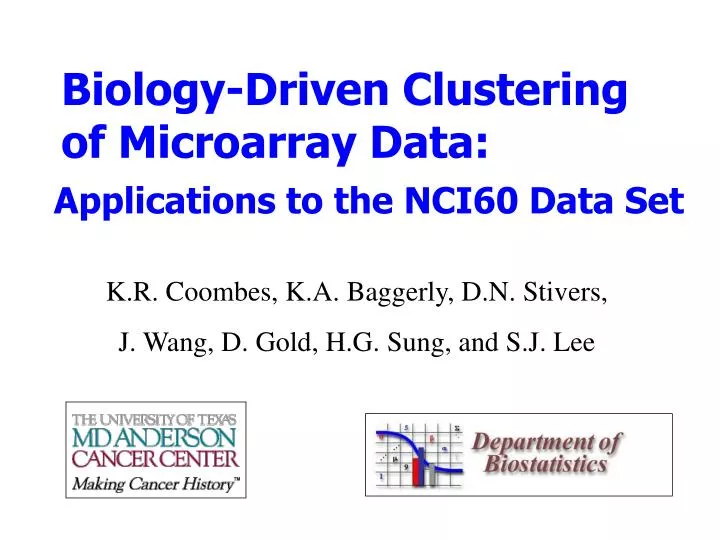
Biology-Driven Clustering of Microarray Data:. K.R. Coombes, K.A. Baggerly, D.N. Stivers, J. Wang, D. Gold, H.G. Sung, and S.J. Lee. Applications to the NCI60 Data Set.

E N D
Biology-Driven Clustering of Microarray Data: K.R. Coombes, K.A. Baggerly, D.N. Stivers, J. Wang, D. Gold, H.G. Sung, and S.J. Lee Applications to the NCI60 Data Set
Most analyses of microarray data proceed as though it were simply a large, unstructured matrix. Such analyses ignore substantial amounts of existing biological information. In the study of cancer, we already know many important genes through their involvement in specific biological processes, and we know that reproducible chromosomal abnormalities play an important role. We see a need for developing analytic strategies that exploit this biological information. We analyzed the NCI60 data set by first determining the chromosomal location and biological function of the genes on the microarray. We performed separate analyses using genes on individual chromosomes and genes involved in different biological processes. The fundamental advantage of this approach is that it provides results that are immediately and directly interpretable without resorting to ex post facto rationalizations. Introduction Methods
Problem: I.M.A.G.E. clone IDs and GenBank accession numbers are archival. UniGene clusters, gene names, descriptions, etc., are changeable. Solution: Download the latest version of UniGene (build 137) and LocusLink (July 2001) to update annotations, using the GenBank accession numbers describing both 3’ and 5’ ends of the genes spotted on the microarrays. How many genes on the microarray have good annotations? Table 1: There are only 7478 spots (out of 10,000) on the array with valid, matching UniGene cluster IDs. Genes with unknown or conflicting annotations were eliminated before performing any further analysis.
Where are the genes located? We compared the number of genes on the microarray that mapped to each chromosome with the number known to be on the chromosome, based on current figures from the NCBI. A chi-squared test was used to test whether the distribution of genes on chromosomes was uniform. Figure 1: Distribution of the genes on the array by chromosome. Chromosomes 19 and Y are substantially underrepresented when compared to the numbers known to LocusLink; chromosomes 6 and 13 are overrepresented.
Using our updated UniGene clusters, we followed the links from UniGene to LocusLink to GeneOntology. GeneOntology is a structured, hierarchical vocabulary to describe gene functions in three broad areas: biological process (why) molecular function (what) cellular component (where) The 7478 good spots on the array corresponded to 6614 distinct genes, of which 5074 were known to LocusLink, and 2989 had at least one annotation in GeneOntology. We focused on the biological process annotations in the GeneOntology vocabulary, since these had the most natural interpretation for application to the study of cancer. We counted the number of genes having annotations of functions at or below each level in the hierarchy, and selected a set of categories that each contained roughly one to a few hundred genes, with the categories as a whole accounting for more than 95% of all annotations (Table 2). How do we determine gene functions?
What functional categories are represented on the array? Table 2: The number of annotations (Ann.) into and the number of spots on the array in various functional categories chosen from the biological process annotations from LocusLink into GeneOntology. Individual spots may have multiple annotations into the same category; individual genes may be represented by multiple spots.
0.6 0.4 0.2 0.0 ovarian.4 ovarian.3 ovarian.5 cns.u251 ovarian.8 nsclc.h23 cns.sf539 cns.sf268 cns.sf295 renal.tk10 cns.snb75 cns.snb19 nsclc.ekvx colon.ht29 renal.a498 renal.786o renal.uo31 renal.achn renal.caki1 nsclc.h460 nsclc.h522 nsclc.h322 nsclc.a549 nsclc.h226 breast.t47d colon.hct15 colon.km12 renal.sn12c breast.mcf7 renal.rxf393 nsclc.hop92 nsclc.hop62 prostate.pc3 colon.sw620 breast.bt549 breast.mdan colon.hct116 breast.hs578t leukemia.hl60 colon.colo205 ovarian.skov3 ovarian.igrov1 leukemia.k562 colon.hcc2998 prostate.du145 leukemia.molt4 melanoma.m14 breast.unknown leukemia.ccrfcem melanoma.loximvi leukemia.srcl7019 breast.mdamb231 breast.mdamb435 melanoma.skmel2 melanoma.skmel5 melanoma.uacc62 leukemia.rpmi8226 melanoma.skmel28 melanoma.uacc577 melanoma.malme3m How good is a dendrogram? We introduced a quality grade, based on the dendrograms, to describe how well each set of genes used to produce a dendrogram classifies each kind of cancer: • A = there is a cluster containing all and only one kind of cancer • B = all, with one or two extras • C = all except one • D = all except one, with extras • E = all except two • F = all except two, with extras Grades for the dendrogram of Figure 2 are displayed in the following table. Figure 2: Dendrogram using all genes with valid annotations and with expression levels above those of the blank spots.
Heterogeneity of different types of cancer • Some cancers (colon, leukemia) are fairly homogeneous and easy to distinguish from others. • Some (breast, lung) are so heterogeneous as to be nearly impossible to distinguish. • Some chromosomes (1, 2, 6, 7, 9, 12, 17) can distinguish many types of cancer. • Some (16, 21) can not accurately distinguish any kind of cancer. The dendrograms using genes from these chromosomes are equivalent to randomly scrambling of the cancer cell lines. Table 3:Grades given to dendrograms that cluster samples by genes on specific chromosomes. Grades range from A to F, with blanks indicating no clustering for that type of sample. Abbreviations: B=breast, C=colon, L=leukemia, M=melanoma, N=non small cell lung, O=ovarian, P=prostate, R=renal, S=central nervous system.
0.6 0.4 0.2 0.0 cns.u251 ovarian.8 ovarian.5 ovarian.3 ovarian.4 nsclc.h23 cns.sf268 cns.sf295 cns.sf539 renal.tk10 cns.snb19 cns.snb75 colon.ht29 nsclc.ekvx renal.uo31 renal.achn renal.a498 renal.786o nsclc.h460 nsclc.h226 renal.caki1 nsclc.h522 nsclc.h322 nsclc.a549 breast.t47d colon.km12 colon.hct15 renal.sn12c breast.mcf7 renal.rxf393 nsclc.hop92 nsclc.hop62 prostate.pc3 colon.sw620 breast.bt549 breast.mdan colon.hct116 breast.hs578t leukemia.hl60 colon.colo205 ovarian.skov3 ovarian.igrov1 leukemia.k562 colon.hcc2998 prostate.du145 leukemia.molt4 melanoma.m14 breast.unknown leukemia.ccrfcem melanoma.loximvi leukemia.srcl7019 breast.mdamb231 breast.mdamb435 melanoma.skmel2 melanoma.skmel5 melanoma.uacc62 leukemia.rpmi8226 melanoma.skmel28 melanoma.uacc577 melanoma.malme3m Chromosome 2 Figure 3: The genes on chromosome 2 do an excellent job of distinguishing cancer types. We can also locate specific clusters of genes on the chromosome with strong signatures identifying leukemia, melanoma, and colon cancer.
0.6 0.4 0.2 0.0 ovarian.8 cns.u251 ovarian.3 ovarian.5 ovarian.4 nsclc.h23 cns.sf295 cns.sf268 cns.sf539 renal.tk10 cns.snb19 cns.snb75 colon.ht29 nsclc.ekvx renal.786o renal.achn renal.a498 renal.uo31 nsclc.h460 nsclc.h226 renal.caki1 nsclc.h322 nsclc.a549 nsclc.h522 breast.t47d colon.hct15 colon.km12 renal.sn12c breast.mcf7 renal.rxf393 nsclc.hop62 nsclc.hop92 colon.sw620 prostate.pc3 breast.bt549 breast.mdan colon.hct116 breast.hs578t colon.colo205 leukemia.hl60 ovarian.skov3 ovarian.igrov1 colon.hcc2998 leukemia.k562 prostate.du145 leukemia.molt4 melanoma.m14 breast.unknown leukemia.ccrfcem melanoma.loximvi leukemia.srcl7019 breast.mdamb435 breast.mdamb231 melanoma.skmel2 melanoma.skmel5 melanoma.uacc62 leukemia.rpmi8226 melanoma.skmel28 melanoma.uacc577 melanoma.malme3m Chromosome 16 Figure 4: Genes on chromosome 16 cannot reliably distinguish any single kind of cancer in this study. There are, nevertheless, strong gene signatures driving the clustering, which does not appear to match anything we know about the biology of the samples.
0.6 0.4 0.2 0.0 ovarian.4 ovarian.5 ovarian.3 ovarian.8 cns.u251 nsclc.h23 cns.sf539 cns.sf295 cns.sf268 renal.tk10 cns.snb75 cns.snb19 colon.ht29 nsclc.ekvx renal.a498 renal.786o renal.achn renal.uo31 nsclc.h522 renal.caki1 nsclc.h322 nsclc.a549 nsclc.h460 nsclc.h226 breast.t47d colon.km12 colon.hct15 renal.sn12c breast.mcf7 renal.rxf393 nsclc.hop62 nsclc.hop92 colon.sw620 prostate.pc3 breast.bt549 breast.mdan colon.hct116 breast.hs578t leukemia.hl60 colon.colo205 ovarian.skov3 ovarian.igrov1 leukemia.k562 colon.hcc2998 prostate.du145 leukemia.molt4 melanoma.m14 breast.unknown leukemia.ccrfcem melanoma.loximvi leukemia.srcl7019 breast.mdamb435 breast.mdamb231 melanoma.skmel2 melanoma.skmel5 melanoma.uacc62 leukemia.rpmi8226 melanoma.skmel28 melanoma.uacc577 melanoma.malme3m Protein Metabolism Figure 5: The genes involved in protein metabolism do an excellent job of distinguishing cancer types. We can also locate specific clusters of genes on the chromosome with strong signatures identifying leukemia, colon cancer, lung cancer, and central nervous system cancer.
0.6 0.4 0.2 0.0 ovarian.3 ovarian.5 cns.u251 ovarian.4 ovarian.8 nsclc.h23 cns.sf295 cns.sf539 cns.sf268 renal.tk10 cns.snb19 cns.snb75 colon.ht29 nsclc.ekvx renal.uo31 renal.a498 renal.786o renal.achn nsclc.h522 nsclc.a549 nsclc.h460 nsclc.h322 renal.caki1 nsclc.h226 breast.t47d colon.km12 colon.hct15 renal.sn12c breast.mcf7 renal.rxf393 nsclc.hop62 nsclc.hop92 colon.sw620 prostate.pc3 breast.bt549 breast.mdan colon.hct116 breast.hs578t colon.colo205 leukemia.hl60 ovarian.skov3 ovarian.igrov1 colon.hcc2998 leukemia.k562 prostate.du145 leukemia.molt4 melanoma.m14 breast.unknown leukemia.ccrfcem melanoma.loximvi leukemia.srcl7019 breast.mdamb231 breast.mdamb435 melanoma.skmel2 melanoma.skmel5 melanoma.uacc62 leukemia.rpmi8226 melanoma.skmel28 melanoma.uacc577 melanoma.malme3m Apoptosis Figure 6: The genes involved in apoptosis do a poor job of distinguishing cancer types. This suggests that the mechanisms by which cancers overcome cell death cut across the normal biological lines drawn by histology.
Multiple views into the data provide substantial insight into differences in cancer types and gene sets. Cancer types differ greatly in their degree of heterogeneity, ranging from homogeneous (colon, leukemia) through moderately heterogeneous (renal, melanoma) to extremely heterogeneous (breast and lung). Homogeneous cancers exhibit strong identifying signals across most views of the data, regardless of function or chromosome. There are large difference in the ability of genes of different chromosomes to distinguish cancer types. There are similar differences for genes involved in different biological processes (data not shown). Functional categories that are good at distinguishing cancers include signal transduction, cell cycle, cell proliferation, and protein metabolism. Some differences result from the histology of the underlying tissue. Others reflect differences in the way particular kinds of cancers overcome limits on cell growth. Categories that are poor at distinguishing cancers include energy pathways and apoptosis. The latter observation has potential implications for cancer therapies designed to trigger apoptosis, since it suggests that the mechanisms by which cancer cells avoid cell death are not linked to the general type of cancer but are either common across cancers or idiosyncratic. Conclusions