Download
1 / 32
371 likes | 991 Views
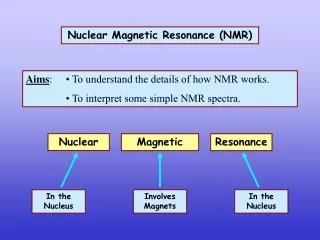
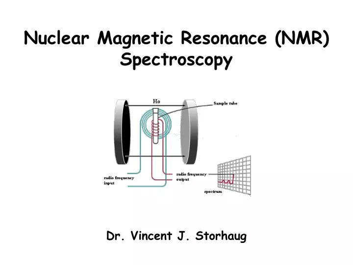
Nuclear Magnetic Resonance (NMR) Spectroscopy. Dr. Vincent J. Storhaug. 2-D NMR Techniques. Defining 2-D NMR techniques:

E N D
Nuclear Magnetic Resonance (NMR) Spectroscopy Dr. Vincent J. Storhaug
2-D NMR Techniques Defining 2-D NMR techniques: • In the following techniques, a number of transients (i.e. – simple 1-D spectra) are taken one after another, with some acquisition parameter (acqpar) being varied SYSTEMATICALLY from one transient to the next. • Since each transient is a collection of digitized data points in the first dimension (say 10 points to make a spectrum) if 10 spectra are accumulated with an incremental change in one acquisition parameter, a Fourier Transform can be performed in the remaining dimension. . . . . . . . . . . . . . . . . . . . . . . . . . . . . . . . . . . . . . . . . . . . . . . . . . . . . . . . . . . . . . . . . . . . . . . . . . . . . . . . . . . . . . . . . . . . . . . . . . . . . . . . . . . . . . . . . . . . . . . . . . . . . . . . . . . . . . . . . . . . . . . . . . . . . . . . . . . . . . . . . . . . . . . . . . . . . . . . . . . . . . . . . . . . . . . . . . . . . . . . . . . . . . . . . . . . . . . . . . . . . . . . . . . . . . . . . . . . . . . . . . . . . . . . . . . . . . . . . . . . . . . . . . . . . . . . . . . . . . . . . . . . . . . . . . . . . . . . . . . . . . . . . . . . . . . . . . . . . . . . . . . . . . . . . . . . . . . . . . . . . . . . . . . . . . . . . . . . . . . . . . . . . . . . . . . . . . . . . . . . . . . . . . . . . . . . . . . . . . . . . . . . . . . . . . . . . . . . . . . . . . . . . . . . . . . . . . . . . . . . . . . . . . . . . . . . . . . . . . . . . . . . . . . . . . . . . . . . . . . . . . . . . . . . . . . . . . . . . . . . . . . . . . . . . . . . . . . . . . . . . . . . . . . . . . . . . . . . . . . . . 1-D FID 1-D spectra, with an incremental variable change FTs can be performed on the vertical data sets
2-D NMR Techniques • Nomenclature: • The first perturbation of the system (pulse) is called the preparation of the • spin system. • The effects of this pulse are allowed to coalesce; this is known as the • evolution time, t1 (NOT T1 – the relaxation time) • During this time, a mixing event, in which information from one part of the • spin system is relayed to other parts, occurs • Finally, an acquisition period as with all 1-D experiments. • Graphically: Preparation Evolution Mixing Acquisition t1
2-D NMR Techniques • COSY: COrrelation SpectroscopY (COSY): • COSY is a HOMONUCLEAR 2-D Technique • A 90° pulse in the y-direction is what we used for 1-D 1H NMR • Here, after a variable “mixing” period, a 90° pulse in the x-direction is • performed, followed by acquisition of a spectrum 90x 90y d1 delay 1 at acquisition time pw1 d2 delay 2 pw2 “t1” time 5*T1
COSY: What Happens at Differing Evolution Times A(t1) t1 t1 wo f2 (t2) Now, we have frequency data in one axis (f2, which came from t2), and time domain data in the other (t1). Since the variation of the amplitude in the t1 domain is also periodic, we can build a pseudo FID if we look at the points for each of the frequencies or lines in f2
COSY: Example Molecules Codeine
COSY: • Performing an experiment on a real molecule • Here is the “real” COSY spectrum: • Observe how this is cumbersome to use in the 3rd dimension • The spectrum is converted to a “contour plot” similar to a flat map of a mountainous region....
2-D NMR: Considerations of Total Acquisition Time 90x 90y d1 delay 1 at acquisition time pw1 d2 delay 2 pw2 “t1” time 5*T1 Let’s say that the T1 is about 3.2 s: then the d1 would be about 15 seconds, and the time required to acquire the transient is about 2.5 seconds. If we need 16 scans for every t1 value, and the average t1 is 300 ms, for ni = 128, we have a total acquisition time of: We have two choices for improving resolution: Improve along f1 or f2. Let’s say we improve along f1 by doubling the number of points in the spectrum (i.e. – we double the acquisition time):
2-D NMR: Considerations of Total Acquisition Time 90x 90y d1 delay 1 at acquisition time pw1 d2 delay 2 pw2 “t1” time 5*T1 Let’s say that the T1 is about 3.2 s: then the d1 would be about 15 seconds, and the time required to acquire the transient is about 2.5 seconds. If we need 16 scans for every t1 value, and the average t1 is 300 ms, for ni = 128, we have a total acquisition time of: We have two choices for improving resolution: Improve along f1 or f2. Let’s say we improve along f2 by doubling the number increments. Then,
Unknown Determinations Involving COSY C13H16O2 You have the chemical formula, so let’s determine the levels of unsaturation:There are 13 carbons, and 14 hydrogens (and we don’t consider oxygens in the calculation, so… The total number of double bonds and/or rings is 6!
Unknown Determinations Involving COSY C7H7NO2 You have the chemical formula, so let’s determine the levels of unsaturation:There are 7 carbons, and 7 hydrogens (and we don’t consider oxygens in the calculation, so… The total number of double bonds and/or rings is 5!
NOESY: Nuclear Overhauser Effect Spectroscopy Unlike the COSY experiment, obtaining good NOESY spectra requires proper values of 90° pulse width and a consideration of delay times. If 90° pulse is incorrect, many “COSY type” (i.e. antiphase cross-peaks) appear, complicating the analysis. In small molecules, some “COSY-type” cross-peaks may be unavoidable even when everything is carefully calibrated. Fortunately these can be easily distinguished because of their antiphase nature, i.e. - the cross-peaks have both positive and negative components but true NOE peaks are pure absorptive. The NOESY experiment must be interpreted more carefully than the COSY experiment because cross-peaks arise from COSY interaction as well as dipolar interaction.
Usefulness of a NOESY The reaction of a bis(spirodienone) calix[4]arene derivative with hydrazine Flavio Grynszpan and Silvio E. Biali Department of Organic Chemistry, The Hebrew University of Jerusalem, Jerusalem 91904, Israel
HETCOR: • Also called _1H-13C COSY – HETeronuclear CORrelation spectroscopy • The only difference on the spectral end, is that one axis is a 13C spectrum • From this data, you can identify which protons are bound to which carbons; again for simple structures this method is unnecessary, but for complex compounds, it is essential
HETCOR: • Also called _1H-13C COSY – HETeronuclear CORrelation spectroscopy • Revisiting our previous example (trans-ethyl 2-butenoate)
Other Methods: • This lecture is by no means thorough; it is meant to give a “taste” of the power and specialization of advanced methods • Here is a compilation of other things that are routinely done; anyone with a knowledge of NMR theory can always devise a new experiment to see something unique! First the 1-D techniques:
Other Methods: • 2-D Methods and Applications
Experimental Practical #1: Digital Resolution Digital Resolution (Hz) Acquisition Time (s) Number of Points in the Fourier Transformed Spectrum Spectral Window (Sweep Width) (Hz)
Experimental Practical #2: Zero Filling Have NOT improved (or worsened) the signal to noise ratio. Have NOT improved (or worsened) the true natural lineshape of the signals. HAVE improved the digital resolution of the observed spectrum.