Revealed Preference Techniques – Cont’d

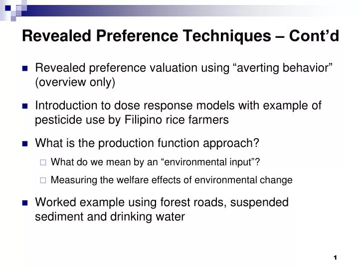
1. Revealed Preference Techniques – Cont’d • Revealed preference valuation using “averting behavior” (overview only) • Introduction to dose response models with example of pesticide use by Filipino rice farmers • What is the production function approach? • What do we mean by an “environmental input”? • Measuring the welfare effects of environmental change • Worked example using forest roads, suspended sediment and drinking water

2. Revealed preference: Averting behaviour Averting behavior infers values from defensive, mitigating, or averting expenditures that prevent or counteract effects of environmental degradation For example, an individual might purchase a water filter to avoid the health risks associated with unfiltered water By analyzing the expenditures associated with these defensive purchases, researchers impute a value to small changes in damage risks Requires understanding of the technical relationship between environmental service and market good substitute Not as useful for valuing ecosystem services since focus is more on health risks (e.g. water quality)

3. Conditions for averting expenditures to produce true welfare measure: Too good to be true? AE must not be a “joint product”; that is, must not generate other benefits as well AE must be a perfect “substitute” for the change in environmental quality Change in AE must be entirely due to the change in environmental quality None of the inputs producing the environmental benefit (e.g. groundwater, well equipment) can be directly valued for themselves AE must not produce a “durable” benefit outlasting the pollution problem itself

4. Dose Response Valuation Method • Usually used to value damages from pollution • Relies on estimation of an emissions damage function • Steps in the process of estimating this function: • measure emissions • determine the resulting ambient environmental quality • estimate human exposure • measure impacts (health, aesthetic, recreation, etc.) • estimate the values of these impacts • Steps 1 & 2 involve the use of diffusion models and are primarily the concern of physical scientists • Linking steps 3 & 4 involves the dose-response function • Step 5 is where economists and valuation tools are used

5. Dose Response method: example • Pingaliet al. (1994) used the dose-response approach to value incremental health costs of pesticide use amongst rice farmers in the Philippines • The variables included were related to spraying and individual characteristics: • age • smoking and drinking habits • weight-to-height ratio • number of herbicide sprays per year • number of pesticide sprays per year

6. Estimated Dose Response Function (Pingaliet al. 1994) • The equation estimated by Pingaliet al was: ln (health cost) = 4.366 + 1.192 x ln(age) - 0.0756 x (ratio of weight to height) + 0.916 x (smoking dummy) - 0.53 x (drinking dummy) + 0.486 x ln(insecticide dose) - 0.042 x ln(herbicide dose) • R2 = 0.30, Degrees of freedom = 100 • The incremental health cost to the average sprayer was: • 1300 pesos per year (US $52) for 4 sprays/year, and • 2070 pesos (US $83) for 8 sprays/year

7. Production Function Approaches to Valuation • Production functions model the contribution of various inputs to outputs in a production process • An ecosystem service may be one of these inputs, e.g. a coastal mangrove area may support commercial fish reproduction • Production function techniques allow the analyst to isolate and value the contribution to output from the environment • If the production process involves complex natural relationships (e.g. fisheries), then a bioeconomic model is needed

8. Establishing the Relationship between Environmental Input and Value A simple PF model involves specifying an output (y) and a vector of purchased inputs (x), along with the environmental input (q): y = f (x,q). As a first approximation of the value of the environmental input, we can take the partial derivative for q: ∂y/∂q = g(x,q) = MPq(marginal product of q) Multiplying by the price, we get the marginal revenue product, MRPq, as a first approximation of value

9. Deriving Welfare Measures of Environmental Change • For proper welfare measures of the value of environmental change, we use the output demand curve and supply curve • Can construct an inverse factor demand curve for the environmental input, assuming that other inputs are held constant • Assuming diminishing returns, this would produce a downward sloping demand curve indicating MRP at different levels of q. • Another view involves the cost side and changes in costs • Changes in the environmental input shift the supply (MC) curve and from this information, changes in consumers' and producers' surplus can be derived

10. Measuring welfare change from an improvement in an environmental input (E) from E0 to E1 Discussion question: What is the change in (i) consumers surplus, (ii) producers surplus, (iii) aggregate welfare? Change in CS is: a gain of a + b + c Change in PS is: a loss of a and a gain of d + e Aggregate welfare change is b + c + d + e

11. Break

12. Ashley Page, Duncan Knowler and Andy Cooper School of Resource and Environmental Management , Simon Fraser University, Burnaby BC Valuing the Water Purification Service of Temperate Rainforests in Coastal British Columbia

13. Outline • Project Background • Study Area • Modeling Approach • Economic Model • Parameter Estimation • Results • Conclusion (Knowler and Dust, 2008)

14. Project Background • Healthy forest ecosystems regulate water quantity and quality • Forestry has an impact on this ecosystem service • Logging road construction can cause sedimentation (turbidity) and its severity is influenced by: • - road density • - traffic volume • Degraded water quality can increase the cost of producing safe drinking water

15. Study Area • NCCW (Norrish Creek Community Watershed) • Multiple-use watershed • Long history of active logging • Drinking water source for over 156,000 BC residents Fraser Timer Supply Area

16. Modeling Approach (II) Key water supply modeling assumptions: • water utility treats raw water and sells treated water at P = AC • if raw water quality (turbidity) exceeds a threshold (10 NTU), alternative high cost sources are used (e.g. groundwater wells) • water quality ‘events’ (> 10 NTU) are a stochastic (count) process influenced by weather & the logging road network

17. Modeling Approach (III) • Welfare analysis compares logging with no logging in the NCCW • Consider four logging & road use scenarios describing the NCCW over a 100 year planning horizon: • logging according to the current forest harvest management plan (Sutherland et al., 2007) with low/moderate/heavy road use variants, and • cessation of all logging within the NCCW

18. Economic Model (I) • Cost function of the water utility with environmental parameter λ (mean water quality ‘events’/week): • Environmental parameter relationship (λ) : where Qis treated water produced in year t, l is length of the road network, u is fixed sediment yield per road km and iis the forest management scenario

19. Economic Model (II) • Demand curve with constant elasticity of demand (Є): → • Supply curve for a water utility pricing at average cost:

20. Economic Model (III) • Unit variable costs are [event (Ve) vs non-event (Vne)]: • Equilibrium water supply Q*is determined by P = AC:

21. Economic Model (III) • Unit variable costs are [event (Ve) vs non-event (Vne)]: • At P = AC, equilibrium water supply Q*for scenario i is:

22. Economic Model (IV) • Change in welfare with a shift from λ0(logging scenario) toλ1(no logging scenario) is: • But there is no producer surplus …

23. Modeling Approach (I) Water utilities: increasing returns and environmental input Welfare gain from improved water quality under an average cost pricing approach

24. Environmental Parameter Estimation (I) Baseline water quality and discharge data for the NCCW Raw turbidity data (1998 – 2002) Raw discharge data (1984 – 2006)

25. Environmental Parameter Estimation (II) Simulated baseline water quality for Norrish Creek Community Watershed using linear mixed-effects models, for various management scenarios and based on 1984 to 2006 historic data, with 10 NTU threshold 19

26. Environmental Parameter Estimation (III) Fitting of the Poisson and Negative Binomial Distributions with estimation of the mean number of times a water quality threshold is surpassed per week, by forest management scenario (λ)

27. Economic Parameters Representative Water Utility Operating Costs % Annual Operating Cost (Conrad et al. 2010)

28. Results (I) Equilibrium prices (P*) and quantities (Q*) of treated water used in welfare analysis for the Logging and No Logging scenarios by level of road use and assuming average cost pricing and a 100 year planning horizon (2008 prices)

29. Results (II) Mean annual change in consumer surplus when shifting from a Logging Scenario to No Logging in the NCCW, assuming a 100 year planning horizon and amortization of capital at 4% (2008 prices)

30. Conclusions • Highlights trade-offs between ecosystem service provision and consumptive uses of forests • We can value this service but need to recognize the complex, stochastic physical processes involved • Research tool to help improve integrated water resource management, especially with climate change • Traffic volumes should be subjected to more regulation in source watersheds