Download
1 / 32
320 likes | 380 Views
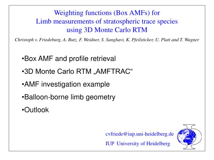
Weighting functions (Box AMFs) for Limb measurements of stratospheric trace species using 3D Monte Carlo RTM Christoph v. Friedeburg, A. Butz, F. Weidner, S. Sanghavi, K. Pfeilsticker, U. Platt and T. Wagner. Box AMF and profile retrieval 3D Monte Carlo RTM „AMFTRAC“

E N D
Weighting functions (Box AMFs) for Limb measurements of stratospheric trace species using 3D Monte Carlo RTM Christoph v. Friedeburg, A. Butz, F. Weidner, S. Sanghavi, K. Pfeilsticker, U. Platt and T. Wagner • Box AMF and profile retrieval • 3D Monte Carlo RTM „AMFTRAC“ • AMF investigation example • Balloon-borne limb geometry • Outlook cvfriede@iup.uni-heidelberg.de IUP University of Heidelberg
Box AMF and profile retrieval • SCD and AMF do not tell us where along the light path the trace gas is located • But this is what we’d like to know. • Discretization of atmosphere into boxes i=1,..,n • SCD box-wise • AMF box-wise: A(i) • Weighting Function • S(i) = c(i) * d(i) • V(i) = c(i) * v(i) • S(i) = V(i) * A(i) • SCD = Σ S(i) • SCD = Σ c(i) * v(i)* A (i) • => into equation system Altd [m] c(i),σ(c,i) d(i) v(i) C [cm-3]
Box AMF and profile retrieval • Box AMF defined as: • sum over all intensity having traversed the layer/cell • divided by total intensity received by detector • divided by layer‘s/cell‘s vertical extension Altd [m] c(i),σ(c,i) d(i) v(i) C [cm-3]
Box AMF and profile retrieval • Multiple scattering increases retrieval difficulty since • geometrical approximations/estimations not valid and misleading • AMF and A(i) must be modelled with RTM • Behaviour of A(i) with relevant parameters must be investigated & understood θ ε
3D Monte Carlo RTM „AMFTRAC“ (working title) e.g. v. Friedeburg EGS 2002 • features • spherical 3D geometry • supports arbitrary platform positions and viewing geometries • full MS by Rayleigh, aerosols, clouds, albedo • refraction, polarization and solar CLD (limb) • principle • backward Monte Carlo technique • N photon launched out of telescope • random numbers, scatt. centre ND & c/s govern light path => establish path sun->detector • molecular absorption calculated analytically • AMF computed from modelled av. intensity with/without absorber ai vv,i di detector
3D Monte Carlo RTM „AMFTRAC“ output • SCDs, SODs, AMFs, Box AMFs (A(i)) for a specified set of boxes/layers • abs. radiances • geometrical path length, traversed air column, O4 • number of Rayleigh, Mie and albedo scattering events • altitudes of first and last scattering event, distance detector-last scattering event • entry angle of light into atmosphere, first scattering angle • Solar CLD effect parameter, polarization (under testing) • parameters as intensity weighted means • errors as intensity weighted std dev.
3D Monte Carlo RTM „AMFTRAC“ radiance validation • In addition to validation against AMF by other RTMs: • validation against measurements with calibrated spectro-radiometer
AMF investigation example ground based MAX DOAS scenario • λ = 352 nm • atmosphere: 1 km vertical discret., 0-70 km • ε = 2°, 5°, 10°, 20°, 45°, 90°; • azimuth α to sun 90°, aperture 0.1° • albedo values 0%, 30%, 50%, 70% • standard aerosol scenario • BrO near ground: 3 profiles investigation of total AMFs in relation to scattering parameters
AMF investigation example BrO AMF P1,P2: AMF highest for 2° elev. P3:?
Results: AMF AMF->f(Albedo), O4 AMF • P3: AMF increases with albedo, but behaviour pertains: • AMF for smallest elevations not highest • same effect for O4 - looks like P1 & 2, but higher proportion (~3/4) located above 1 km.
AMF investigation example Number of scatterings • Single scattering approx. („1/sin(τ)“, „1/cos(θ)“) heavily limited • similar investigations for higher wavelengths useful
AMF investigation example Last Scattering Altitude LSA LSA • LSA for small elevations between 300 and 400 m • =>decreases light path within lowest boxes as comp. to 1/sin(ε)
AMF investigation example LSA -> AMF(i) LSA • LSA for small elevations < 1 km • A(i) for boxes above 1 km decrease for low elevations
Balloon-borne limb geometry • relevant to SCIAVAL balloon operations • SCIAMACHY limb mode • SZA (at altd 0 below instrument position): 70° • atmosph. discret. 1 km • Variation of • altitude • elevation angle • azimuth angle • aperture angle • cloud cover
Balloon-borne limb geometry Error investigation • Box AMF error’s absolute value depends on: • Number of paths • layer’s/grid cell’s shape & extension • layer’s/grid cell’s distances from the instrument • influence of multiple scattering on the way to & within the layer • incl. albedo, clouds • 2000 PU was used for the calculations to follow.
Balloon-borne limb geometry Altitude variation • Line Of Sight Parameters: • -4° elevation, 90° azimuth, 0.5° aperture, 30% albedo • above instrument: Box AMF governed by SZA • below instrument: Box AMF increases due to LOS geometry, • at altd<25 km LOS hits ground • below altitude of highest Box AMF: fall-off depends on aperture (see aperture var.) • near ground AMFs dependent on multiple scattering
Balloon-borne limb geometry Altitude variation: scattering parameters • NRS (MS importance) decreases with increasing altitude • Last Scattering Distance (LSD) affected by MS • LSA complies well with altitude of highest Box AMF
Balloon-borne limb geometry Elevation variation • LOS Parameters: • 90° azimuth, 0.5° aperture, altitudes 10 and 30 km • strong variation in sensitivity for tangent altitude • tangent altitude moves upwards • important for limb scanning geometry - total Box AMF as weighted average • below tangent altitude Box AMF largely unaffected
Balloon-borne limb geometry Elevation variation • LOS Parameters: • 90° azimuth, 0.5° aperture, altitudes 10 and 30 km • strong variation in sensitivity for tangent altitude • tangent altitude moves upwards • important for limb scanning geometry - total Box AMF as weighted average • below tangent altitude Box AMF largely unaffected
Balloon-borne limb geometry Azimuth variation • LOS Parameters: • -4° elevation, 90° azimuth, 0.5° aperture, altitudes 10 and 30 km • impact small as compared to e.g. elevation influence • for az. 90° Box-AMF largest in tangent alt, above for az 180° “sun beam” has to travel longer distance to reach LOS intersection point
Balloon-borne limb geometry Aperture variation • LOS Parameters: • -4° elevation, 90° azimuth, 0.5° aperture, altitudes 10 km • fall-off below tangent altd influenced by aperture for geometrical reasons • for ap. angles <1° effect small but: • depends on chosen discretization • changing elevation (scanning) equals a higher effective ap. angle
Balloon-borne limb geometry Cloud cover variation • LOS Parameters: • -4° elevation, 90° azimuth, 0.5° aperture, altitudes 10 and 30 km • cloud cover: • 1. grid cell filled with Mie particles - high CPU time • 2. layer with altitude, coverage, albedo, transmission • multiple layers, vertical cloud surfaces easy to implement • accuracy depends on cloud effects impact on measurement • cloud layer altitude 5 km albedo 80%, transmission zero
Balloon-borne limb geometry Cloud cover variation: O4, radiance • LOS Parameters: • -4° elevation, 90° azimuth, 0.5° aperture, altitude 10 km • radiance: smooth increase with cloud cover • O4: decrease due to lower troposphere shielding
Conclusion/Outlook • AMFTRAC capable of handling limb geometry in relevant LOS parameters • output parameters help understanding AMF‘s and A(i)‘s behaviour quantitatively • Investigation of use of polarization and CLD effects • Implementation of realistic clouds and aerosols • Inclusion of basic LES-based retrieval module
MAX-DOAS, AMF and profile retrieval • DOAS: Differential Optical Absorption Spectroscopy • Measured quantity: optical density τ of trace gases investigated • integrated over light path • σ(λ) absorption cross section c(s) concentration • along “slant” light path : Slant Column Density SCD = τ(λ) / σ(λ) • along vertical path from location: Vertical Column Density VCD • related by Air Mass Factor AMF • VCD=SCD / AMF • Measure of sensitivity • for the trace gas profile
MAX-DOAS, AMF and profile retrieval • Solar light enters atmosphere on straight path • gets scattered by e.g. Rayleigh, Mie, albedo • enters telescope => AMFs depend on: • Solar Zenith Angle (SZA θ) and Solar Azimuth Angle • scattering centre number density, cross section, phase fct. • elevation ε, aperture angle,... θ ε
Investigation: Influence of aerosol how to retrieve aerosol data - radiance? • radiance series R(ε) : Spectrographs not usually absolutely calibrated • dR/dε not significantly different to allow for concl. on aerosol
Investigation: Influence of aerosol LSA • without aerosol impact effect present, but much weaker • aerosol scenario largely governs AMF -> f(ε) • use of std. scen. Risky => need hard data on local aerosol
Investigation: Influence of aerosol albedo in many cases known; aerosol load not. investigation on AMF->f(aerosol) for albedo 30%
Investigation: Influence of aerosol how to retrieve aerosol data - O4? • But O4-AMF->f(ε) signif.tly different for large aerosol ld. differences • parametrize the O4-AMF(ε) behaviour as f(aerosol ext. coeff.) => scale aerosol ext. coeff. • uncertainties: effect of phase function ?
MAX model scenario • aerosols: • continental scenario (F. Hendrick, IASB, pers. comm.) • ext. coeff. Value for 0 km varied for investigation
Monte Carlo Approach for MS • calculation of distance d to next voxel boundary • extinctors (Rayleigh, Mie particles) yield probability p(x) for free passage up to x • p(d)=p0 prob. of unscattered passage along d • map random number p‘ to x by the inverse of function p(x): • determines location of scattering event [0,d] • use a second random number to decide between scatterers according to the relative probabilities d p‘ 1 p0 Xd