Download
1 / 40
420 likes | 545 Views
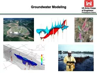
Use of Information on Hydrologic Extremes : US Army Corps of Engineers Perspective. Beth Faber, PhD, PE USACE, IWR, Hydrologic Engineering Center Statistical Assessment of Extreme Weather Phenomena under Climate Change Boulder, CO June 13-17, 2011. USACE Mission Areas.

E N D
Use of Information on Hydrologic Extremes: US Army Corps of Engineers Perspective Beth Faber, PhD, PE USACE, IWR, Hydrologic Engineering Center Statistical Assessment of Extreme Weather Phenomena under Climate Change Boulder, CO June 13-17, 2011
USACE Mission Areas • The US Army Corps of Engineers has a “mission” in several areas of water management • Most deal with streamflow, some with average annual volumes, some with extremes (high or low) • Flood Risk Management • Ecosystem Restoration • Navigation (inland, coastal) • Water Supply • Hydropower • Recreation concerned with extreme HIGH flows concerned with sea level concerned with annual flow volumes concerned with extreme LOW flows
USACE “Response” to Climate Change • Our understanding of our hydrologic environments and how we describe them must account for change over time, that is difficult to predict • formerly, used the past variability to describe future variability • and, we’re accustomed to predictable change in that variability… • Corps’ response to climate change is mainly in two areas • Decision-making • how we incorporate a new kind of uncertainty • Data(to inform decision-making) • how we describe the environments the public exists within (inland hydrology, storms, sea-level)
Data, and use of data • I’m going to show what data we use, how we summarize it, and how it enters our decision-making • local-scale daily hydrology, or daily temp/precip • What we need to know from climate scientists: • How can we evaluate climate change impact on extremes? • What are the climate models good at? What aren’t they good at? • What outputs have value, that we can base decisions on? • How should we down-scale spatially and temporally? • What’s the meaning of the model “ensemble”? Does it span the uncertainty? Does it capture the distribution of uncertainty?
Natural Variability • We’re used to dealing with natural variability • Our projects are designed to perform for the range of hydrology • Describe hydrology by both annual statistics and by probability distributions of extreme events (frequency curves) • Questions for climate scientists and statisticians: • Have the observed climate trends exceeded the range of natural variability? • At what point would the plausible climate futures exceed the natural variability (or change it)? • How can we estimate the variability of the future?
Decision-making • We’re accustomed to making decisions with uncertain info • All of our hydrologic statistics and modeling are uncertain • Decisions span a reasonable range of the uncertainty • But, decisions that span very large uncertainty and array of possible outcomes become less effective • Now focused on adaptive decision-making (hedge and adjust) • Robust actions that are acceptable for a range of outcomes • Staged decisions that are revisited and adjusted over time • Decisions that don’t exclude other future actions or avenues • The life-span of a decision affects the uncertainty included • Uncertain info, want to reduce the impact of being wrong
USACE Mission Areas • The US Army Corps of Engineers has a “mission” in several areas of water management • Most deal with streamflow, some with average annual volumes, some with extremes (high or low) • Flood Risk Management • Ecosystem Restoration • Navigation (inland, coastal) • Water Supply • Hydropower • Recreation concerned with extreme HIGH flows concerned with sea level concerned with annual flow volumes concerned with extreme LOW flows
Biggest Issue – Extreme Highs • The Corps’ most prominent mission area is flood risk management • Formerly referred to as “flood control” or “flood damage reduction” • The new term reflects a new way of thinking and making decisions about flood risk • More about getting out of the way than changing or blocking the flow, and consciously addressing the risk • For flood risk management, the most important input to characterize hydrology is the probability distribution of annual peak flows (flood-frequency curve)
Flood Risk Management • Risk analysis and risk managementrequire estimates of the probability of extreme events with negative consequences • Risk = Probability × Consequence • Need a relationship between flood magnitude and annual exceedanceprobability • might differ for the present and the planning horizon • This relationship allows us to perform probabilistic analyses involving high streamflows and their consequences (damage, lives lost)
Typical Flood Frequency Curve Return Period 2 5 10 25 50 100 200 500 EXTREME Log Scale 90% confidence interval Normal Probability Scale
Flood Frequency Analysis • When possible, we infer probability from a record of annual maximum observations (Bulletin 17B) • using the past variability as a representation of the future • use LogPearson type III distribution (least wrong for 100yr event) • Treat annual peak flows as a random, representative sample of realizations from the flood population of interest • Generally, we assume the sample is IID • annual peak flows are random and independent • peak flows are identically distributed – homogeneous data set • sample is adequately representative of the population • These assumptions are becoming more difficult…
Generation of the Flood Frequency Curve Return Period 2 5 10 25 50 100 200 500 1903 – 2009 109 years Log Scale LogPearson III Normal Probability Scale
Uncertainty in the Flood Frequency Curve Return Period 2 5 10 25 50 100 200 500 1965 – 2009 45 years Log Scale Normal Probability Scale
Corps Activities that require Flood-Frequency • Corps of Engineers responsibilities involve both water management and development of infrastructure • Make decisions based on probabilistic analysis, and where possible, explicit incorporation of uncertainty • … uncertainty in probabilistic estimates of flow, and uncertainty in other modeling (hydrologic, hydraulic and economic) • We use the probabilistic description of flooding in: • Safety of projects • Scale of projects (and updated “performance”) • Operation of projects
Safety of Projects levees, dams, locks, ports, hydropower • In the past, required that projects can withstand the occurrence of the Probable Maximum Flood (PMF) without failure (e.g., sizing of spillway) • note: capacity exceedance ≠ failure • Now, we evaluate overall risk (exceedanceOR failure), and target a tolerable riskto remain below • Risk = probability of occurrence × consequence • Evaluate all possible failure modes and their likelihoods, as well as the likelihoods of loading thresholds (from the flood-frequency curve)
Dynamics of Likelihood vs. Consequences: • original estimate of risk • risk management implemented • probability: strengthen, raise capacity • consequence: remove structures • due to aging and wear&tear • due to climate change? • due to maintenance, repairs, and improved operations • resulting from development pressure • on-going risk management activities • Land use management • Flood proofing • Warnings and preparedness plans Tolerable Risk Limit 1 3 Likelihood 2 6 5 4 Consequences 16
Scale of Projects • This is the “Planning” function • Federal dollars are spent to provide an equal or greater benefit to the Nation • formerly, the explicit benefit of a project was a reduction in annualized flood damage (levees, dams, “non-structural” actions) • now, also incorporate reduction in loss of life • Projects are scaled (sized) such that either net benefits (benefit – cost) or benefit/cost ratioare maximized • no defined target, but now must be below tolerable risk limit • Annualized benefit is the reduction in mean annual damage (or, EAD), based on the probability distribution of peak annual flow
Computing EAD with summary curves • EAD = Expected Annual Damage • The probability distribution of annual flood damage for a river reach is computed by combining summary curves developed from hydrologic frequency, hydraulic and economic analyses: flow-frequency curve to obtain a: flow-stagecurve damage-frequencycurve stage-damagecurve • The mean of the damage-frequency curve is the expected value of annual damage, or EAD.
AREA = mean = Expected Annual Damage Computing EAD with summary curves F(Q) Flow (cfs) Peak Flow (cfs) 0 p 1 Stage (ft) Exceedance Probability F(D) Damage ($) Damage ($) p 0 1 Stage (ft) Exceedance Probability
Uncertainty in EAD Use Monte Carlo simulation to sample many realizations of each curve to compute many realizations of EAD F(Q) Flow (cfs) Peak Flow (cfs) 0 p 1 Stage (ft) Exceedance Probability F(D) Damage ($) Damage ($) AREA = mean = Expected Annual Damage p 0 1 Stage (ft) Exceedance Probability
Project Performance • Another measure for project scale is the performance of the project, and how it might change over time • Project performance is a combination of the likelihood of capacity exceedance and the likelihood of failure • A flood protection project is designed having a certain probability of capacity exceedance • a change in the flood-frequency curve causes a change in the probability of capacity exceedance • This change might cause a difference with regard to the National Flood Insurance Program
90% conditional non-exceedance probability for the 1%-chance event… 90% 100-year Levee Certification 60 55 50 45 40 35 30 25 20 estimated stage-frequency curve
Operation of Projects • This is the Corps’ Water Management function • Reservoirs have Guide Curves (GC) that specify the upper bound of storage • Below GC is Conservation space for storing water for later use • navigation, hydropower, water supply, flow maintenance, flow temperature control, (and recreation – don’t use!) • Above GC is Flood space for storing flood flows • Store flood volume until can release safely downstream • Either maintain a flood pool, or draft enough space to store forecasted snowmelt flood
flood benefitsare proportional to flood volume Guide Curve supply benefits are proportional to supply volume Reservoir Storage Pools An increase in the flood-frequency curve would let existing flood pool offer less protection (larger chance exceedance), or require a larger flood pool More variability in flow, or a decrease in average annual volume would decrease the yield of the Conservation pool Flood Pool Conservation Pool A decrease the low-flow frequency curve would require more yield for streamflow maintenance
Seasonal Reservoir Pools • Get more benefit to each use when have more volume serving it – so multi-use space is efficient • When there’s a limited flood season, or only snowmelt runoff flooding, use seasonal pools • A seasonal Guide Curve calls for a flood pool during part of the year, and allows it to fill when there is little or no probability of flooding • a change in the flood season would require changing GC • When only snowmelt runoff flooding (Pacific Northwest), draft a flood pool volume based on runoff forecasts
Seasonal Flood Pool – Rain Flooding Convenient timing: snowmelt starts when rainy season ends, catch volume. What if earlier snowmelt runoff before rain-flood season is over? Guide Curve flood pool flood volume snowmelt runoff Reservoir Volume conservation pool Guide Curve supply volume rain flood season Oct Jul Apr Jan Oct
Seasonal Flood Pool – Rain Flooding Convenient timing: snowmelt starts when rainy season ends, catch volume. What if earlier snowmelt runoff before rain-flood season is over? Guide Curve flood pool flood volume snowmelt runoff Reservoir Volume conservation pool Guide Curve supply volume rain flood season Oct Jul Apr Jan Oct
Seasonal Flood Pool – Snowmelt Flooding With snowmelt forecast, draft enough to catch flood peak. But some forecasts are based on historical record… Guide Curve flood pool flood volume snowmelt runoff Reservoir Volume Variable Guide Curves conservation pool supply volume snowmelt flood season Oct Jul Apr Jan Oct
Frequency Analysis, non-stationarity • Standard (B17B) frequency analysis assumes data is IID (independent and identically distributed) • use the past to estimate likelihood for the future • Some change can be dealt with, if the change is recognizable and predictable • example: urbanization • adjust earlier flood peak data to current basin condition • KEY: the trend must be observable to be removed, and predictable to have an estimate of a future condition • Climate change/trend is more difficult to recognize, more difficult to predict
Return Period 2 5 10 25 50 100 200 500 Adjustment for Urbanization
Decisions under uncertainty • How can we address this increased uncertainty about future hydrology? • There are two opposite approaches: • Find a way to make better estimates of the future • Work with the uncertainty. Make decisions (project scaling, operation plans) more robust(able to perform well in a wider array of conditions) and able to adapt as change is recognized (realized) • NOTE: adaptation is quite feasible for project operations, but less so for infrastructure development. Plan for staged development of infrastructure, but more costly in the end
How can we do better frequency analysis? • If our gaged flood records are not IID, how should we do frequency analysis? • Fit parameters that vary as a function of time? • Other covariates? • Attempt to adjust all historical floods to an estimated present or future condition? • Run climate models longer to capture a stationary (current or future) condition? • Attempt frequency analysis on shorter periods?
Return Period 2 5 10 25 50 100 200 500 1909 – 2011 103 years
Return Period 2 5 10 25 50 100 200 500
Return Period 2 5 10 25 50 100 200 500
Return Period 2 5 10 25 50 100 200 500 Random 30-year Samples from full-period Frequency Curve
Short-record Frequency Curves • It’s difficult to make assumptions based on frequency curves from short records • The uncertainty in those short-record frequency curves overwhelms any change we might see in the short-term • Need more data to infer probability distributions, to reduce uncertainty so that it’s less than the change due to climate.