Download
1 / 38
380 likes | 532 Views
y. x. 0. Definitions. Coordinate systems and dimensions The objects considered in Computational Geometry are points, lines, line segments, polygons, polyhedron, hyper-rctacgles etc. A coordinate system provides a means to specify positions or points in space.

E N D
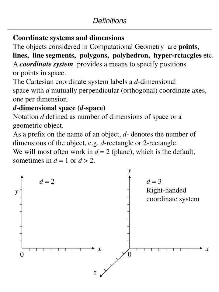
y x 0 Definitions Coordinate systems and dimensions The objects considered in Computational Geometry are points, lines, line segments, polygons, polyhedron, hyper-rctacgles etc. A coordinate system provides a means to specify positions or points in space. The Cartesian coordinate system labels a d-dimensional space with d mutually perpendicular (orthogonal) coordinate axes, one per dimension. d-dimensional space (d-space) Notation d defined as number of dimensions of space or a geometric object. As a prefix on the name of an object, d- denotes the number of dimensions of the object, e.g. d-rectangle or 2-rectangle. We will most often work in d = 2 (plane), which is the default, sometimes in d = 1 or d > 2. d = 2 d = 3 Right-handed coordinate system y x 0 z
p0 p1 p0 Definitions Point Object with d dimensions and 0 extent. Location in d-space. Given as an ordered sequence of d coordinates. d = 1 (x) or x d = 2 (x, y) d = 3 (x, y, z) d 4 (x1, x2, ..., xd) or (x0, x1, ..., xd-1) Line Infinite “straight” 1-dimensional set of points, determined by two points p0, p1p0p1.
p1 p0 p1 p0 Definitions Segment Finite 1-dimensional subset of a line, determined by two endpoints p0, p1. Ray Infinite 1-dimensional subset of a line determined by two points p0, p1p0p1, where one point is denoted as the endpoint.
Preliminaries Point-Line classification We now consider the geometric primitive operation of classifying a point w.r.t. a line (both in the plane). A directed line segment partitions the plane into 7 non-overlapping regions. The possibilities are shown below. The problem, given p0, p1, and p2, is to determine which region p2 lies in. beyond p1 left terminus between p0 origin right behind
< 0 p1 = 0 0< < 1 p0 = 1 > 1 Preliminaries Parametric equation of a line We use the following equation of a line: line = {(p0) + (1 - (p1) }, where (real numbers) where p0 and p1 as usual are the points determining the line. p0 = (x0, y0) p1 = (x1, y1) Substituting gives {(x0, y0) + (1 - (x1, y1) } Multiplying through gives the coordinates {x0 + (1 - x1, y0 + (1 - y1 } Work out an example with points (4,3) and (7,5) as the two end points with values of as 0, 1, 0.5, 2 and -3. For example, when equal to 2 , (x,y)=(2 x0 – x1 , 2 y0 - y1 ) = (1,1).
Line Segment A line segment is a closed subset of a line contained between two points which are called the end points. The subset is closed in the sense that it includes the end points. The equation of the line segment is the same as the parametric equation of a line with the restriction that has the value 01. This is also called the convex combination of the two end points.
Explicit Form of Line Equation y= mx +c m=slope=tan where is the angle made by the line with positive x-axis c=intercept of the line with the y-axis. Vertical line with x=k cannot be represented since these lines have infinite slopes. Expressed in terms of the coordinates of two points on the line (x1,y1) and (x2,y2), we can write y=[(y2-y1)/(x2-x1)] x + (y1x2 -y2x1)/(x2-x1) Or (x2-x1)(y-y1)= (y2-y1)(x-x1) This is called an implicitform of an equation of a line. Now, x2=x1 and y2y1 means a vertical line with equation x=x1. y m=tan c x
In general, a line equation in a plane can be specified as Ax + By + C = 0 where A, B and C are constants. A vertical line is simply a line with B=0. Note the coefficients are not unique; for a given constant k, kA, kB and kC will give the same line. In general, in a d-dimension, given a set of k points p1,p2,..,pk, the set of points p= 1 p1+ 2 p2+….+ k pk such that the -coefficients are real and their sum equals 1, is called an affine combination of the given set of k points . For k=2, this set defines a straight line through two points; for k=3, it is a plane and for higher k value it is called a hyperplane.
p2 p1 p0 Definitions Plane Infinite 2-dimensional subset of space, determined by three points p0, p1, p2, p0p1p2 p0. Interval Pair of coordinate values. Often treated like a segment on a coordinate axis. [l, r] closed; xlxr is within interval (l, r) open; xl < x < r is within interval [l, r) half open; xlx<r. (l, r] half open; xl<xr is within interval l r closed 0 l r open 0
We will use degrees or radians, as convenient. 90 y x 0 Definitions Rectangle Quadrilateral with opposite sides parallel and only right angles. Rectilinear or axis-parallel rectangle Cartesian product of d intervals. 2-rectangle or simply rectangle
Definitions Dimensional prefixes on geometric object names No prefix “d-” means usual or expected number of dimensions for the object. rectangle = 2-rectangle cube = 3-cube Prefix “hyper-” means d is unspecified and it may be more than the usual number of dimensions for that object. hyper-rectangle = d-rectangle, d unspecified “d-dimensional rectilinear hyper-rectangle”
Definition --------------------------------------------------------- Polygon: In two dimensions, it is defined by a finite set of line segments such that every point (vertex) is shared by two line segments (edges) and no subset of the segments has the same property. Example: Individually each collection of line segments is a Polygon, but taken together it is not a polygon since it violates the subset property. Simple Polygon: A polygon is simple if there are no points between non-consecutive line segments, that is, vertices are the only intersection points. In the above diagram, the first two are simple polygons But the third one is not. The following is not even a Polygon:
Note a non-simple polygon may be drawn alternately as a planar “graph” but as drawn it is still not a simple polygon 4 1 2 3 3 2 1 5 4 5 Non-simple polygon Corresponding planar graph In computational geometry, the relative geometrical positions and dimensions matter. The “edges” do not represent an abstract “relation” as in graph theory.
Definitions Polygons O’Rourke, pp. 1-2 A polygon is the region of a plane bounded by a finite set of segments forming a simple closed curve. (Note that we are working in d = 2 by definition.) Let v0, v1, ..., vN-1 be N points in the plane; the points are called vertices. Let e0 = v0v1, e1 = v1v2, ..., eN-1 = vN-1v0 be N segments connecting the points; the segments are called edges. The edges bound a polygon iff the intersection of each pair of edges adjacent in the ordering is the single vertex shared between them: eiei+1 = vi+1 for i = 0, N - 1 v4 v5 v3 N = 8 v6 v2 v7 v0 v1 Vertices are numbered in counterclockwise sequence by convention.
Boundary Interior Definitions The segmentsare connected end-to-end in a sort of a curve, they form a cycle and hence it is closed, and the closed curve is simple since non-adjacent segments do not intersect. We also have this famous theorem: Interior and exterior Jordan curve theorem. Every simple closed plane curve divides the plane into two parts. Exterior Polygon = interior boundary If we are interested in just the interior or just the boundary, they will be referred to as such. (Same as true for other similar objects, e.g., rectangle.). The two parts are called the exterior (unbounded) and the interior (bounded). Thus the polygon P is the region of a plane bounded by a finite collection of line segments forming a simple closed curve. Sometimes a polygon is considered to be just the segments bounding the region and not the region itself. This is defined as P. Thus, P P.
Definitions Polygon Not vertices Simple polygon A polygon is simple iff non-adjacent edges do not intersect. eiej = for all 0 j, i N - 1 and ji + 1.
Definitions Convex polygon A polygon is convex if and only if for any two points in the polygon (interior boundary) the segment connecting the points is entirely within the polygon. convex not convex
CONVEX SET Let p and q be two arbitrary points in a d-dimensional Euclidean space belonging to a set of points C. Then C is said to be convex if for all pairs (p,q) in C, the set of points [p + (1- )q] C for 0<= <=1 That is, if two pints p and q belong to C, then the set of points on the line segments connecting p and q also belong to C. When d=2, the points belong to a convex polgon.
Planar Graph A graph G(V,E) is palnar if it can be embedded in a plane without crossings. ( Kuratowski’s Theorem: no “subgraph “ or homomorphic to the subgraphs: A straight line planar embedding of a planar graph determines a partition of the plane called planar subdivisions or a map. Let v= number of vertices, e= number of edges and f=number of faces. Theorem ( Euler) : v - e + f = 2 Proof: A smple polygon has always v=e and f=2 ( interior and exterior).
If the interior is further subdivided by a chord, it creates one extra face. V remains same, e becomes e+1 and f becomes f+1. So the equation remains valid. If a chain is used with t new vertices and necessarily with t+1 edges, we have v becomes v+t, e becomes e+t+1 and f becomes f+1. So, the Euler’s formula still remains valid. chain chord It can also be shown that for any planar graph, e <= 3v -6. Using Euler’s formula, we then have f<= 2/3 e and f <= 2v-4, giving the upper bounds on f in terms of e and v, respectively. Furthermore, if for each vertex v>= 3 ( polyhedron) then, 3v<=2e which yields e<= 3f-6 and v<=2f-4. All these relations are linear.
POLYHEDRON In 3-d Euclidean space, a polyhedron is defined to be a finite set of planar polygons such that every edge of the polygon is shared by exactly one other neighboring polygon and no subset of polygons has the same property ( to avoid union of polygons). Edges and vertices have usual meaning. The polygons are called the facets of the polyhedron. A polyhedron is simple if there is no pair of non-adjacent facets sharing a point. A simple polyhedron partitions the 3-d space into two disjoint domains - the interior and the exterior. A simple polyhedron is convex if its interior is convex. The surface of a polyhedron is isomorphic to a planar subdivision ( on a sphere). Thus the numbers v, e and f of a simple polyhedron obey Euler’s formula.
Definitions Vertices A polygon vertex is convex if its interior angle It is reflex if its interior angle > reflex convex In a convex polygon, all the vertices are convex.
Computational Model ----------------------------------------------------------------- Human brains perform complex geometrical computations using a model not yet understood. We certainly don’t use floating point numbers! Neural networks attempt to mimic very poorly the actions of the brain cells – but in the process again introduces “numbers” as weights! Nature computes with molecules and atoms, not numbers. The great enigma is that human brain invented mathematics which is supposed to be independent of nature. Ironically, mathematics was invented to explain nature! We are stuck with the RAM ( Random Access Memory) model in our computation but we modify the model by assuming that each cell in the memory can hold a number of infinite precision. This is a very powerful model since it isolates geometry from the details of computation. Thus, we can say that the computation of intersection of two points, which may not be identified by any rational numbers in some cases, takes constant amount of time.
----------------------------------------------------------- In practice, we do indeed take constant time for such a computation by introducing computational errors, which may multiply, propagate, proliferate ultimately creating a non-sense computation. For example: Draw a “complete” graph on 5 vertices as on a plane such that the boundary is a convex 5-gon. You will see an “inner” pentagon. Repeat this process. If computers have to carry on this process, after several iterations, all the points will become “fuzzy” and inaccurate. The study of errors in computational geometry and solid modeling and its impact on the models that you create for simulation is a research topic that has attracted many reserachers.
Preliminaries Example problem RANGE SEARCHINGGiven N points in the plane, how many lie in a given rectangle with sides parallel to the coordinate axes? That is, how many points (x, y) satisfy lx x rx, ly y ry, for given lx rx, ly ry? ry ly lx rx The range searching problem is (informally) defined above. In this example, the instance of the range searching problem is a particular set of points and a particular range. In an instance like this, the points are the data set.
Preliminaries Algorithms and models of computation We are interested in efficient algorithm for geometric problems. Efficiency is evaluated in terms of computational cost, given as a function of the size of the instance of the problem. By convention, notation N denotes input instance size. To determine the computational cost of an algorithm, we must know what primitive operations are available and what they cost. This is a model of computation. Turing machine: too primitive C language on Unix workstation: too specific We will use a highly abstract model, the familiar random-access machine from [Aho,1974]. We use a slightly modified real RAM model. These operations are available at unit cost: 1. arithmetic; +, -, *, / 2. comparisons; <, , =, , , > 3. memory access 4. analytic functions; root, trig, exp, log Numbers are assumed to be real, with infinite precision. This is considerably abstracted; in a real machine: 1. different operations vary widely in cost 2. floating point precision is limited You must deal with the latter in your code. The abstract model of computation allows us to focus on how computation cost changes w.r.t. input instance size.
Preliminaries Order notation We are interested in the amount of time and memory used by algorithms, as a function of the input instance size N. “Worst case” or Upper bound O(f(N)) denotes the set of all functions g(N) such that there exist positive constants C and N0 with g(N) Cf(N) for all NN0. “Best case” or Lower Bound (f(N)) denotes the set of all functions g(N) such that there exist positive constants C and N0 with g(N) Cf(N) for all NN0. “Optimal case” Or Optimal Bound (f(N)) denotes the set of all functions g(N) such that there exist positive constants C1, C2, and N0 with C1f(N) g(N) C2f(N) for all NN0. Notes: These notations denote sets: f(N) O(log N), not f(N) = O(log N). Larger terms dominate the order, e.g., (4N + 20 log N + 100) O(N) We will use the notation for both time and memory. Most of our attention will be towards “worst case”.
Preliminaries Example analysis SEGMENT INTERSECTION COUNTING INSTANCE: Set S = {s1, s2, ..., sN} of line segments in the plane. QUESTION: Count the number of intersections of segments in S.
Preliminaries Example analysis SEGMENT INTERSECTION COUNTING INSTANCE: Set S = {s1, s2, ..., sN} of line segments in the plane. QUESTION: Count the number of intersections of segments in S. 1 procedure SegmentIntersectionCounting(S) 2 begin 3 count = 0 3 for i = 1 to N 4 for j = 1 to N 5 if ij and sisj 6 count = count + 1 7 endif 8 endfor 9 endfor 10 print count 11 end Storage: O(N), for set S Time: O(N2), for nested loops Notice the assumed primitive operation: segment intersection. What geometric operations are primitive?
Preliminaries Algorithmic complexity measures Preprocessing. Time spent organizing the data set, usually into some data structure. Less important than query and storage. Query. Time spent producing the answer for a query relative to the data set. Storage. Memory required for static and dynamic data structures used by the query algorithm. Single shot vs. repetitive-mode Single shot. Given a single data set and a single query, produce ananswer one time. Almost always best handled by scan of data set; no preprocessing, query O(N), storage O(N). Repetitive-mode. Given a single data set and a sequence of queries, produce the answer for each query relative to the data set. Here we are willing to spend time preprocessing to enable query time better than O(N).
Preliminaries Counting vs. reporting Counting. Determine the number of objects in the data set that satisfy the query. Reporting. Report (list, identify) the objects that satisfy the query. For example, consider the standard range search problem: RANGE SEARCHING. INSTANCE: Set S = {p1, p2, ..., pN}, pi = (xi, yi) of points in the plane, and rectangle R = [lx, rx] [ly, ry] in the plane. QUESTION (counting): How many points of S are within R? QUESTION (reporting): Which points of S are within R?
Preliminaries Output sensitive or report-mode algorithms The time complexity of algorithms is often expressed as a function of input data set size, e.g. O(N log N). Reportingproblems can have query time complexity that is output sensitive. Output-sensitive example INTERVAL ENCLOSURE INSTANCE: Set S = {x1, x2, ..., xN} of points on the number line (x-axis), and an interval Q = [l, r]. QUESTION: Which points of S are within Q, i.e. l xir? Naive repetitive mode algorithm and analysis. Preprocessing: 1. Sort S into an array A. O(N log N) Query: 1. Binary search A for xil. O(log N) 2. Binary search A for xjr. O(log N) 3. Report points from xi to xj in A. ? There can be O(N) points from l to r step 3 is O(N) query is O(N). Without reporting, query is O(log N), with reporting O(N). Time complexity of this type is usually written O(log N + K), where N is input size and K is output size.
Average Complexity: observed complexity in practice. Space or Storage Complexity. Pre-processing Cost: trade-off between space and time complexity with or without pre-processing . Amortized Cost: average over expensive and inexpensive operations. Normalization It will sometimes be useful to have available normalized values for coordinates. For a coordinate value x, its normalized x coordinate is in [1, N], assigned in order of increasing x coordinate, relative to the set from which the coordinates are/will be drawn. Normalization usually implies an O(N log N) sort in preprocessing and O(log N) normalization search in query.
Preliminaries Segment Tree A segment tree is a rooted binary tree that stores data intervals onthe real line whose extremes (endpoints) belong to a fixed set of N abscissae (x-values). It is the set of x-values from which the endpoints are chosen that is fixed, not the intervals themselves. The tree structure in which the intervals are stored is defined for a scope interval [l, r]. For a given [l, r] there is exactly one segment tree structure. The data intervals are stored within the fixed tree. We will assume WLOG that the data interval endpoints have been normalized to [1, N] and the tree has been built for scope interval [1, N]. T(l, r) = Segment tree over scope interval [l, r]. Each node v of T(l, r) is associated with a scope interval [l, r]. A node v has these parameters: B(v) Beginning of scope interval associated with this node. E(v) End of scope interval associated with this node. Lchild(v) Left subtree = T(B(v), (B(v) + E(v)) / 2) Rchild(v) Right subtree = T((B(v) + E(v)) / 2E(v)) A(v) List of data intervals stored (“allocated”) to this node. [B(v), E(v)) is the scope interval associated with node v. It is closed on the left and open on the right (except nodes on the rightmost path of T, which are closed on both ends).
[1,12] [1,6) [6,12] [1,3) [3,6) [6,9) [9,11] [7,8) [8,9) [10,11) [11,12] Preliminaries Example The structure of the segment tree T(1,12) is shown. Each node is labeled with its associated interval [B(v), E(v)). [10,12] [4,6) [1,2) [2,3) [3,4) [6,7) [7,9) [9,10) [4,5) [5,6) The set of intervals {[B(v), E(v)) or [B(v), E(v)] v a node of T(l, r)}are the standard intervals of T(l, r). Standard intervals which are also leaves are elementary intervals. These are simply [i, i + 1) for l i < r and [r - 1, r]. T(l, r) is balanced, with depth log(r - l) O(log N).
Preliminaries Insertion The segment tree structure supports insertions and deletions of intervals with endpoints {l, l + 1, l + 2, ..., r}, in O(log N) time per operation. For r - l > 3, an arbitrary interval [b, e] inserted into T(l, r) willbe partitioned into and “allocated” as a collection of standard intervalsof T(l, r). There will be at most log (r - 1) + log (r - 1) - 2O(log N) standard intervals in the partition. To insert interval [b, e] into segment tree T: InsertSegmentTree(b, e, root(T)) procedure InsertSegmentTree(b, e, v) begin if (bB(v) and E(v) e) then add [b, e] to A(v) else if (b < (B(v) + E(v)) / 2 ) then InsertSegmentTree(b, e, Lchild(v)) if ((B(v) + E(v)) / 2 < e) then InsertSegmentTree(b, e, Rchild(v)) end end
[1,12] [1,6) [6,12] [1,3) [6,9) [9,11] [3,6) [4,6) [6,7) [2,3) [7,8) [10,11) [11,12] Preliminaries Example Insertion of [2, 8) into T(1,12): (B(v) + E(v)) / 2 6 3 9 2 4 7 [10,12] 5 6 8 [1,2) [3,4) [7,9) [9,10) 7 [8,9) [4,5) [5,6) Interval [2, 8) allocated to nodes [2, 3), [3, 6), [6, 7), [7,8). An underlying assumption here is that all the intervals inserted and deleted is closed on the left and open on the right. Thus if we have to represent [2,8] we will have to start with [2,9).
Preliminaries Deletion Deletion is symmetric with insertion. To delete interval [b, e] from segment tree T: DeleteSegmentTree(b, e, root(T)) procedure DeleteSegmentTree(b, e, v) begin if (bB(v) and E(v) e) then remove [b, e] from A(v) else if (b < (B(v) + E(v)) / 2 ) then DeleteSegmentTree(b, e, Lchild(v)) if ((B(v) + E(v)) / 2 < e) then DeleteSegmentTree(b, e, Rchild(v)) end end