Download
1 / 25
250 likes | 427 Views
A Mechanistic Model of Mid-Latitude Decadal Climate Variability. (IMAGe T-O-Y Workshop IV). Sergey Kravtsov Department of Mathematical Sciences, UWM May 19, 2006. Collaborators : William Dewar, Pavel Berloff, Michael Ghil, James McWilliams, Andrew Robertson. Multi-scale problem!!!.

E N D
A Mechanistic Model of Mid-Latitude Decadal Climate Variability (IMAGe T-O-Y Workshop IV) Sergey Kravtsov Department of Mathematical Sciences, UWM May 19, 2006 Collaborators: William Dewar, Pavel Berloff, Michael Ghil, James McWilliams, Andrew Robertson
Multi-scale problem!!! North Atlantic Ocean — Atmosphere System: Large-scale (1000 km) high-frequency (monthly) atmospheric patterns vs. small-scale (100 km) low-frequency (interannual) oceanic patterns associated with Gulf Stream variability Atmosphere: some degree of scale separation between synoptic eddies (somewhat smaller and faster) and large-scale low-frequency patterns Ocean: some spatial-scale separation in along-current direction (“eddies” vs. “jet”)
SST and NAO Decadal time scale detected in NAO/SST time series If real, what dynamics does this signal represent? We will emphasize ocean’s dynamical inertia due to eddies AGCMs: response to (small) SSTAs is weak and model-dependent SST tripole pattern (Marshall et al. 2001, Journal of Climate: Vol. 14, No. 7, pp. 1399–1421) Nonlinear: small SSTAs – large response??
Coupled QG Model • Eddy-resolving atmospheric and ocean components, both cha- racterized by vigorous intrinsic variability • (Thermo-) dynamic coupling via constant- depth oceanic mixed layer with entrainment
Atmospheric driving of ocean • Coupled effect: Occupation frequency of atmospheric low-latitude state exhibits (inter)-decadal broad-band periodicity
Eddy effects on O-LFV–I (EPV-flux tendency regressed onto PC-1 of 1) ALL LL HH – 10 yr – 5 yr 0 yr + 5 yr + 10 yr
Eddy effects on O-LFV–II T – “slow” time scale; – “fast” time scale Substitute decomposition into equation and average over slow time scale:
Eddy effects on O-LFV–III – coarse grid “large-scale” solution forced, at the coarse grid, by the history of , where is the fine-grid solution; – “eddy component” O x x x O x x x x x x x x x x x x x x x O x x x O O – coarse grid x – fine grid
Eddy effects on O-LFV–IV • Dynamical decomposition into large-scale flow and eddy-flow components, based on parallel integration of the full and “coarse- grained” ocean models (Berloff 2005) • “Coarse-grained” model forced by randomized spatially-coherent eddy PV fluxes exhibits realistic climatology and variability • Main eddy effect is rectification of oceanic jet (eddy fluctuations are fundamental)
Dynamics of the oscillation–I Initial state A-jet shift O-jet is maintained for a while largely due to stochastic eddy forcing via rectification
Dynamics of the oscillation – II • High Ocean Energy = High- Latitude (HL) O-Jet State • HL ocean state = A-jet’s Low-Latitude (LL) state • O-Jet stays in HL state for a few years due to O-eddies
Dynamics of the oscillation – III • Oscillation’s period is of about 20 yr in low- ocean-drag case and is of about 10 yr in high- ocean-drag case • Period scales as eddy- driven adjustment time
Conceptual model – I • Fit A-jet position time series from A-only simu- lations forced by O-states keyed to phases of the oscillation to a stochastic model of the form [ V(x) – polynomial in x ]
Conceptual model – III “Atmosphere:” “Ocean:” -1=2 yr, Td=5 yr • Delay: ocean’s jet does not “see” the loss of local atmospheric forcing because ocean eddies dominate maintenance of O-jet for as long as Td • Atmospheric potential function responds to oceanic changes instantaneously: O-Jet HL state favors A-Jet LL state and vice versa
Summary • Mid-latitude climate model involving turbulent oceanic and atmospheric components exhibits inter-decadal coupled oscillation • Bimodal character of atmospheric LFV is res- ponsible for atmospheric sensitivity to SSTAs • Ocean responds to changes in occupation frequency of atmospheric regimes with a delay due to ocean eddy effects • Conceptual toy model was used to illustrate how these two effects lead to the coupled oscillation