STATISTICAL ANALYSIS FOR ORIGIN-DESTINATION MATRICES OF TRANSPORT NETWORK

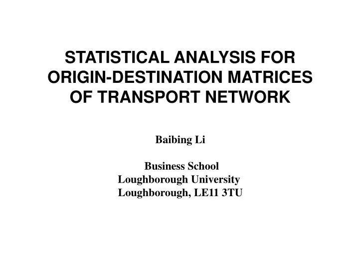
1. STATISTICAL ANALYSIS FOR ORIGIN-DESTINATION MATRICES OF TRANSPORT NETWORK Baibing Li Business School Loughborough University Loughborough, LE11 3TU

2. Overview STATISTICAL ANALYSIS FOR ORIGIN-DESTINATION MATRICES OF TRANSPORT NETWORKS • Background • Statement of the problem • Existing methods • Bayesian analysis via the EM algorithm • A numerical example • Conclusions

3. Example. Located in Northwest Washington, DC, bounded by Loughboro Road in the north; Canal Road and MacArthur Boulevand in the west; and Foxhall Road in the east Canal Road is a principal arterial, two lanes wide, generally running northwest-southeast Foxhall Road is a two-way, two-lanes minor arterial running north-south through the study area Loughboro Road is a two-way east-west road Background

4. What is a transport network A transport network consists of nodes and directedlinks An origin (destination) is a node from (to) which traffic flows start (travel) A path is defined to be a sequence of nodes connected in one direction by links Background

5. Background • Origin-destination (O-D) matrices • An O-D matrix consists of traffic counts from all origins to all destinations • It describes the basic pattern of demand across a network • It provides fundamental information for transport management

6. Background

7. Background • Methods of obtaining O-D data • Roadside interviews and roadside mailback questionnaires disruption of traffic flow; unpopular with drivers and highway authorities • Registration plate matching very susceptible to error (e.g. a vehicle passing two observation points has its plate incorrectly recorded at one of the points) • Use of vantage point observers or video for small study area (e.g. to determine the pattern of flows through a complex intersection) • Traffic counts much cheaper than surveys; much smaller observation errors

8. Statement of the problem • Statement of the problem • Aim: Inference about O-D matrices • Available data: traffic counts A relatively inexpensive method is to collect a single observation of traffic counts on a specific set of network links over a given period

9. Statement of the problem • Notation • y=[y1,…,yc]T is the vector of the traffic counts on all feasible paths(ordered in some arbitrary fashion) • x=[x1,…,xm]T is the vector of the observed traffic counts on the monitored links. • z=[z1,…,zn]T be the vector of O-D traffic counts • The matrix A is an mc path-link incidence matrix for the monitored links only, whose (i, j)th element is 1 if link i forms part of path j; otherwise 0 • The matrix B is an nc matrix whose (i, j)th element is 1 if path j connects O-D pair i; otherwise 0

10. Statement of the problem • Statistical model (I) x = Ay z = By • Assume that y1,…,yc are unobserved independent Poisson random variables with means 1,…,c respectively, i.e. yi~ Poisson(yi; i). Denote =[1,…,c]T • Vector x has a multivariate Poisson distribution with a mean of A

11. Statement of the problem x (monitored link) y123 2 1 3 y423 y43 x=y123+y423 4 z43=y43+y423

12. Statement of the problem • Statistical model (II) x = Pz • P*= [pij] is a proportional assignment matrix, where pij is defined to be the proportions of using link j which connects O-D pair i (assumed to be available).P is a sub-matrix of selecting those rows associated with x • A common assumption is that the O-D counts zjare independent Poisson variates, thus x being linear combinations of the Poisson variates with mean of P, where  is the mean of z

13. Statement of the problem x (monitored link) y123 2 1 3 y423 y43 Note y123=z13 If y423=0.3z43 4 then x=1.0z13+0.3z43

14. Statement of the problem • Relationship between Model (I) and Model (II) Assumptions: • O-D traffic counts zj are independent Poisson random variables with mean j • If yj =[yjk]is vector of route flows and pj=[pjk] route probabilities for O-D pair j, then conditional upon the total number of O-D trips, then yj ~ multinomial(zj, pj) Conclusion: • The distributions of yjkare Poisson with parameters jk =jpjk

15. Statement of the problem • Major research challenges • A highly underspecified problem for inference about an O-D matrix from a single observation • An analytically intractable likelihood

16. Statement of the problem • Example of multivariate Poisson distributions • Let Y1, Y2, and Y3 be three independent Poisson variates Yi~ Poisson(yi; i) • Define X1= Y1+Y3 and X2= Y2+Y3. The joint distribution of X1 and X2is a multivariate Poisson distribution:

17. Previous research • Maximum entropy method (Van Zuylen and Willumsen, 1980) --- Dealing with the issue of under-specification • Maximising entropy, subject to the observation equations • Adding as little information as possible to the knowledge contained in the observation equations

18. Previous research • Using normal approximations (Hazelton, 2001) --- Dealing with intractability of multivariate Poisson distributions To circumvent the problem, Hazelton (2001) considered following multivariate normal approximation for the distribution of y: Since x = Ay, we obtain Note that the covariance matrix  depends on .

19. Bayesian analysis + EM algorithm • Basic idea --- dealing with the issue of intractability Instead of an analysis on the basis of the observed traffic counts x, the inference will be drawn based on unobserved y • Incomplete data • The observed network link traffic counts x are treated as incomplete data (observable) • Follow a multivariate Poisson --- analytically intractable • Complete data • The traffic counts on all feasible paths, y, are treated as complete data (unobservable) • Follow a univariate Poisson --- analytically tractable

20. Bayesian analysis + EM algorithm • Basic idea --- dealing with the issue of under-specification Bayesian analysis combines two sources of information • Prior knowledge e.g. an obsolete O-D matrix; or non-informative prior in the case of no prior information • Current observation on traffic flows

21. Bayesian analysis • Complete-data Bayesian inference • Complete-data likelihood P(y | ) The joint distribution of y: ∏j Poisson(yj |j ) • Incorporate a natural conjugate prior () j ~ Gamma(j; j) • Result in a posterior density P( | y ) j ~ Gamma (aj; bj) with aj=j+ yj and bj=j+1

22. The EM algorithm • Posterior density • Prior density () • Complete-data likelihood P(y | )=P(x | )P(y | x, ) • Complete-data posterior density P( | y )  P(y | )() • E-step: averaging over the conditional distribution of y given (x, (t)) E{logP( | y ) | x, (t) }=l( | x)+E{logP(y | x, ) | x, (t) }+log((t))+c • M-step: choosing the next iterate (t+1)to maximize E{logP( | y ) | x, (t) } Each iteration will increase l( | x) and {(t)} will converge

23. The EM algorithm • Bayesian inference via the EM algorithm • M-step The a posteriori most probable estimate of j is given by (j+ yj1)/(j+1) • E-step Replacing the unobservable data yj by its conditional expectation at the t-th iteration: (j+ E{yj | x, (t)}1)/(j+1)

24. Conditional expectation • Calculation of conditional expectation • Theorem. Suppose that {yj} are independent Poisson random variables with means {j} (j=1,…,c) and A=[A1,,Ac] is an mc matrix with Ajthe jth column of A. Then for a given m1 vector, x, we have E{yj | x, (t)}= j(t) {Pr(Ay=xAj) /Pr(Ay=x)} Major advantage: guarantee positivity

25. Estimation, prediction & reconstruction • Hazelton (2001) has investigated some fundamental issues and clarified some confusion in the inference for O-D matrices. He clearly defines the following concepts: • Estimation The aim is to estimate the expected number of O-D trips • Prediction The aim is to estimate future O-D traffic flows • Reconstruction The aim is to estimate the actual number of trips between each O-D pair that occurred during the observational period

26. Prediction • For future traffic counts, the complete-data posterior predictive distribution is • The complete-data marginal posterior predictive distributions are negative binomial distributions with • The mode of the marginal posterior predictive distribution is at • Given the incomplete data x, the prediction is

27. Reconstruction • The marginal distributions of yj are NB(j ,j). Denote the corresponding probability mass functions as • For given observation x, the reconstructed traffic counts can be calculated as the a posteriori most probable vector of y, i.e. the solution to the following maximization problem: subject to Ay=x • Solving the above problem yields the reconstructed traffic counts

28. A numerical example

29. A numerical example Table A1. Prior estimates of origin-destination counts

30. A numerical example Table A2. True values of origin-destination counts

31. A numerical example • Prior distributions The prior distributions are taken as Gamma distributions with parameters j being the prior estimates in Table A1 and j =1 • Simulated data • Simulation of unobservable vector of traffic counts, y outcomes of independent Poisson variables with means displayed in Table A2. • Monitored links Assume the traffic counts are available on m=8 of the links, i.e. links 1, 2, 5, 6, 7, 8, 11, 12. • Simulation of a single observation,x=Ay x = [884, 548, 111, 133, 191, 144, 214, 640]T.

32. A numerical example

33. A numerical example • Repeated experiments • The simulation experiment was repeated 500 times • The quality of prior information varies via adjusting the parameters of the prior distributions (j; j) with  = 1, 2, 5, 10, 20 ,50 • j* are the ‘true’ values of the parameters in Table A2 and j0are the prior values in Table A1

34. A numerical example

35. Conclusions • Bayesian analysis • Challenge: a highly underspecified problem for inference about an O-D matrix from a single observation • Solution: Bayesian analysis combining the prior information with current observation • The EM algorithm • Challenge: an analytically intractable likelihood of observed data • Solution: the EM algorithm dealing with unobservable complete data which have analytically tractable likelihood

36. References Hazelton, L. M. (2001). Inference for origin-destination matrices: estimation, prediction and reconstruction. Transportation Research, 35B, 667-676. Li, B. (2005). Bayesian inference for origin-destination matrices of transport networks using the EM algorithm. Technometrics, 47, 2005, 399-408. Van Zuylen, H. J. and Willumsen, L. G. (1980). The most likely trip matrix estimated from traffic counts. Transportation Research, 14B, 281-293.