Download
1 / 11
110 likes | 255 Views
Streamflow Predictability. Tom Hopson. Conduct Idealized Predictability Experiments. Document relative importance of uncertainties in basin initial conditions and weather and climate forecasts on streamflow Account for how uncertainties depend on type of forcing (e.g. precip vs. T)

E N D
Streamflow Predictability Tom Hopson
Conduct Idealized Predictability Experiments • Document relative importance of uncertainties in basin initial conditions and weather and climate forecasts on streamflow • Account for how uncertainties depend on • type of forcing (e.g. precip vs. T) • forecast lead-time • Regions, spatial-, and temporal-scales • Potential implications for: • how to focus research efforts (e.g. improvements in hydrologic models vs data assimilation techniques) • observational network resources (e.g. SNOTEL vsraingauge) • anticipate future needs (e.g. changes in weather forecast skill, impacts of climate change)
Initial efforts • Start with SAC lumped model and SNOW-17 • (ignoring spatial variability) • Applied to different regions • Four basins currently • Drive with errors in: • initial soil moisture states (multiplicative) • SWE (multiplicative) • Observations (ppt – multiplicative; T – additive) • Forecasts with parameterized error growth • Place in context of climatological distributions of variables to try and generalize regional and seasonal implications (e.g. forecast error in T less important in August compared to April in snow-dominated basins)
Sources of Predictability Model solutions to the streamflow forecasting problem… Historical Data SNOW-17 / SAC Historical Simulation SWE SM Q Past Future • Run hydrologic model up to the start of the forecast period to estimate basin initial conditions;
Sources of Predictability Model solutions to the streamflow forecasting problem… Historical Data Forecasts SNOW-17 / SAC SNOW-17 / SAC Historical Simulation SWE SM Q Past Future • Run hydrologic model up to the start of the forecast period to estimate basin initial conditions; • Run hydrologic model into the future, using an ensemble of local-scale weather and climate forecasts.
Sacramento Soil Moisture Accounting (SAC-SMA) model Rainfall -Evapotranspiration - Changes in soil moisture storage = Runoff • Physically based conceptual model • Two-layer model • Upper layer: surface and interception storages • Lower layer: deeper soil and ground water storages • Routing: linear reservoir model • Integrated with snow17 model • Model parameters: 16 calibrated parameters • Input data: basin average precipitation (P) and Potential Evapotranspiration (PET) • Output: Channel inflow (Q)
Study site: Greens Bayou river basin in eastern Texas Greens Bayou basin • Drainage area: 178 km2 • Most of the basin is highly • developed • Humid subtropical climate • 890-1300 mm annual rain • Unit Hydrograph: • Length 31hrs, time to conc 5hr DJ Seo
Forcing and state errors • Observed MAP – multiplicative • [0.5, 0.8, 1.0, 1.2, 1.5] • Soil moisture states (up to forecast initialization time) – multiplicative • [0.5, 0.8, 1.0, 1.2, 1.5] • Precipitation forecasts – error growth model
Forecast Error Growth models • Lorenz, 1982 • Primarily IC error E small E large Another options: Displacement / model drift errors: E ~ sqrt(t) (Orrell et al 2001)
Error growth, but with relaxation to climatology Error growth around climatological mean Short-lead forecast Probability/m Longer-lead forecast Climatological PDF => Use simple model Precipitation [m] Where: pf(t) = the forecast prec errstatic = fixed multiplicative error w(t) = error growth curve weight po(t) = observed precip qc = some climatologicalquantile Error growth of extremes Probability/m Errstatic = [0.5, 0.8, 1.0, 1.2, 1.5] qc = [.1, .25, .5, .75, .95] percentiles Precipitation [m]
Greens Bayou Precip forcing fields – Nov 17, 2003 tornado Perturbed soil moisture (up to initialization) All perturbed (including soil moisture) Perturbed obsppt [mm/hr] Perturbed fcstppt Q response [mm/hr] Note: high ppt with low sm (aqua) Low ppt with high sm (green)