Download
1 / 16
160 likes | 350 Views
Physics Labs with Computer Interfaces. Dr. Jing Gao Chemistry and Physics Department Kean University April 12, 2003. Introduction. In our physics lab, student use Pasco’s motion sensor to measure their own position, and velocity with respect to the sensor;

E N D
Physics Labs with Computer Interfaces Dr. Jing Gao Chemistry and Physics Department Kean University April 12, 2003
Introduction In our physics lab, student use Pasco’s • motion sensor to measure their own position, and velocity with respect to the sensor; • DataStudio to curve fit their motion live to a plot given on the computer display. Uniqueness: students are the objects being measured; through direct involvement, they have a better understanding of the physics.
Equipments • Hardware: Science workshop interface 750 (Motion Sensor II) • Software: DataStudio
Motion Sensor II • Ultrasound pulses are sent out and their echoes reflected from an object are detected measuring range: 0.15m<x<8m • Changing in position of an object is measured many times each second. Trigger rate: 5Hz<f<120 Hz • Use the feedback from the ‘cursor’ to locate the best starting position Delay time: t=3s
Understand Motion 1: Position and Time To Interface Motion Sensor
Understand Motion 1: x~t • Study the given plot to determine • How close should you be to the Sensor at start? • How far away should you move? • How long should your motion last? • Data recording • Find best starting point through cursor feedback. • Match your motion to the plot already there. • Repeat several runs to improve the match.
x(m) 4 2 t(s) 0 6 4 2 8 -2 -4 Fig.1 Position as a function of time Given Plot
Motion descriptions: x~t • Starting at 1m from the sensor, • first 2s no motion, • with 1m/s speed away from sensor 3s, • no motion for another 2s, • with 4m/s speed towards sensor for 1s.
x(m) 4 2 t(s) 0 6 4 2 8 -2 -4 Fig.1 Position as a function of time Matching Plots
Understand Motion 2: Velocity and Time To Interface Motion Sensor
Understand Motion 2: v~t • Study the given plot to determine • The direction to go at the beginning; • The maximum speed must achieve; • The Duration of the motion. • Data Recording • Challenge: Match your motion to the plot • The v~t is more erratic than x~t plot.
v(m/s) 4 2 t(s) 0 80 40 60 20 -2 -4 Fig.2 Velocity as a function of time Given Plot
Motion descriptions: v~t • moving with 1m/s speed for first 20s • speed increasing constantly to 4m/s during 20-50s, • moving with const. speed 4m/s for 20s, • speed decreasing constantly to zero for the last 10s
v(m/s) 4 2 t(s) 0 80 40 60 20 -2 -4 Fig.2 Velocity as a function of time Matching Plots
Outcome and discussion • Students are attracted to the technology: very involved and eager to be challenged. • They learn while doing it: gaining better understanding of properties of a motion • Improve their data analysis & computer application skills
Conclusion • DataStudio computer interface labs provide students with a powerful tool in describing and analyzing motion of an object graphically. • Numerous applications in all branches of Physics, as well as other science areas, including Biology, Chemistry, and Earth & Environmental Science.