Download
1 / 40
400 likes | 517 Views
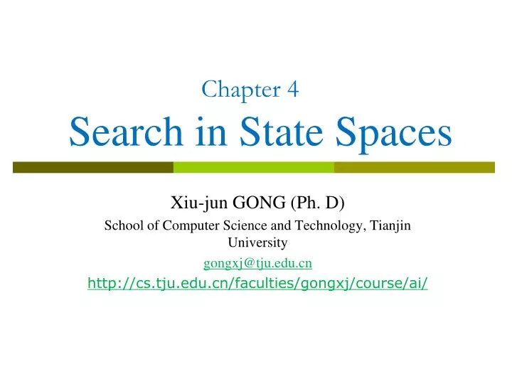
Chapter 4 Search in State Spaces. Xiu-jun GONG (Ph. D) School of Computer Science and Technology, Tianjin University gongxj@tju.edu.cn http:// cs.tju.edu.cn/faculties/gongxj/course/ai /. Outline. Formulating the state space of a problem Strategies for State Space Search

E N D
Chapter 4 Search in State Spaces Xiu-jun GONG (Ph. D) School of Computer Science and Technology, Tianjin University gongxj@tju.edu.cn http://cs.tju.edu.cn/faculties/gongxj/course/ai/
Outline • Formulating the state space of a problem • Strategies for State Space Search • Uninformed search: BFS,DFS • Heuristic Search: A*, Hill-climbing • Adversarial Search: MiniMax • Summary
State Space • a state space is a description of a configuration of discrete states used as a simple model of machines/problems. Formally, it can be defined as a tuple [N, A, S, G] where: • N is a set of states • A is a set of arcs connecting the states • S is a nonempty subset of N that contains start states • G is a nonempty subset of N that contains the goal states.
State space search • State space search is a process used in the field of AI in which successive configurations or states of an instance are considered, with the goal of finding a goal state with a desired property. • State space is implicit • the typical state space graph is much too large to generate and store in memory • nodes are generated as they are explored, and typically discarded thereafter • A solution to an instance may consist of the goal state itself, or of a path from some initial state to the goal state.
Formulating the State Space • Explicit State Space Graph • List all possible states and their transformation • Implicit State Space Graph • State space is described by only essential states and their transformation rules
Explicit State Space Graph • 8-puzzle problem • state description • 3-by-3 array: each cell contains one of 1-8 or blank symbol • two state transition descriptions • 84 moves: one of 1-8 numbers moves up, down, right, or left • 4 moves: one black symbol moves up, down, right, or left
Explicit State Space Graph cont. • The number of nodes in the state-space graph: • 9! ( = 362,880 ) Only small problem can be described by Explicit State-Space Graph Part of State space graph for 8-puzzle
Implicit State Space Graph • Essential States • start: (2, 8, 3, 1, 6, 4, 7, 0, 5) • Goals • (1, 2, 3, 8, 0, 4, 7, 6, 5) • Rules 2 8 3 1 6 4 7 5 1 2 3 8 4 7 6 5
J 0 1 2 I 0 1 2 Implicit State Space Graph cont. Implicit State-Space Graph (rules & essential states) uses less memory than Explicit State-Space Graph • Rules R1: if A(I,J)=0 and J>0 then A(I,J):=A(I,J-1), A(I,J-1):=0 (空格左移) R2: if A(I,J)=0 and I>0 then A(I,J):=A(I-1,J), A(I-1,J):=0 (空格上移) R3: if A(I,J)=0 and J<2 then A(I,J):=A(I,J+1), A(I,J+1):=0 (空格右移) R4: if A(I,J)=0 and I<2 then A(I,J):=A(I+1,J), A(I+1,J):=0 (空格下移)
Search strategy • For huge search space we need, • Careful formulation • Implicit representation of large search graphs • Efficient search method • Uninformed Search • Breadth-first search • Depth-first search • Heuristic Search
Breadth-first search • Advantage • Finds the path of minimal length to the goal. • Disadvantage • Requires the generation and storage of a tree whose size is exponential the depth of the shallowest goal node • Extension • Branch & bound
DFS • Advantage • Low memory size: linear in the depth bound • saves only that part of the search tree consisting of the path currently being explored plus traces • Disadvantage • No guarantee for the minimal state length to goal state • The possibility of having to explore a large part of the search space
Iterative Deepening • Simply put an upper limit on the depth (cost) of paths allowed • Motivation: • e.g. inherent limit on range of a vehicle • tell me all the places I can reach on 10 litres of petrol • prevents search diving into deep solutions • might already have a solution of known depth (cost), but are looking for a shallower (cheaper) one
Iterative Deepening cont • Memory Usage • Same as DFS O(bd) • Time Usage: • Worse than BFS because nodes at each level will be expanded again at each later level • BUT often is not much worse because almost all the effort is at the last level anyway, because trees are “leaf –heavy”
Heuristic Search • Using Evaluation Functions • A General Graph-Searching Algorithm • Algorithm A* • Algorithm description • Admissibility • Consistence
Using Evaluation Functions • Best-first search (BFS) = Heuristic search • proceeds preferentially using heuristics • Basic idea • Heuristic evaluation function : based on information specific to the problem domain • Expand next that node, n, having the smallest value of • Terminate when the node to be expanded next is a goal node • Eight-puzzle • The number of tiles out of places: measure of the goodness of a state description
Using Evaluation Functions cont. A Possible Result of a Heuristic Search Procedure
Using Evaluation Functions cont. • A refine evaluation function
A General Graph-Searching Algorithm • Create a search tree, Tr, with the start node n0 put n0 on ordered list OPEN • Create empty list CLOSED • If OPEN is empty, exit with failure • Select the first node n on OPEN remove it put it on CLOSED • If n is a goal node, exit successfully: obtain solution by tracing a path backward along the arcs from n to n0 in Tr • Expand n, generating a set M of successors + install M as successors of n by creating arcs from n to each member of M • Reorder the list OPEN: by arbitrary scheme or heuristic merit • Go to step 3
A General Graph-Searching Algorithm cont. • Breadth-first search • New nodes are put at the end of OPEN (FIFO) • Nodes are not reordered • Depth-first search • New nodes are put at the beginning of OPEN (LIFO) • Best-first (heuristic) search • OPEN is reordered according to the heuristic merit of the nodes • A* is an example of BFS • The algorithm was first described in 1968 by Peter Hart, Nils Nilsson, and Bertram Raphael.
Algorithm A* • Reorders the nodes on OPEN according to increasing values of • Some additional notation • h(n): the actual cost of the minimal cost path between n and a goal node • g(n): the cost of a minimal cost path from n0 to n • f(n) = g(n) + h(n): the cost of a minimal cost path from n0 to a goal node over all paths via node n • f(n0) = h(n0): the cost of a minimal cost path from n0 to a goal node • estimate of h(n)
Algorithm A* Cont. (Procedures) • Create a search graph, G, consisting solely of the start node, n0 put n0 on a list OPEN • Create a list CLOSED: initially empty • If OPEN is empty, exit with failure • Select the first node on OPEN remove it from OPEN put it on CLOSED: node n • If n is a goal node, exit successfully: obtain solution by tracing a path along the pointers from n to n0 in G • Expand node n, generating the set, M, of its successors that are not already ancestors of n in G install these members of M as successors of n in G
Algorithm A* Cont. (Procedures) • Establish a pointer to n from each of those members of M that were not already in G add these members of M to OPEN for each member, m, redirect its pointer to n if the best path to m found so far is through n for each member of M already on CLOSED, redirect the pointers of each of its descendants in G • Reorder the list OPEN in order of increasing values • Go to step 3
Properties of A* Algorithm • Admissibility • A heuristic is said to be admissible • if it is no more than the lowest-cost path to the goal. • if it never overestimates the cost of reaching the goal. • An admissible heuristic is also known as an optimistic heuristic. • A* is guaranteed to find an optimal path to the goal with the following conditions: • Each node in the graph has a finite number of successors • All arcs in the graph have costs greater than some positive amount • For all nodes in the search graph,
Properties of A* Algorithm cont. • The Consistency (or Monotone) condition • Estimator h holds monotone condition, if (nj is a successor of ni) • A type of triangle inequality
Properties of A* Algorithm cont. • Consistency condition implies • values of the nodes are monotonically nondecreasing as we move away from the start node • Theorem: If on is satisfied with the consistency condition , then when A* expands a node n, it has already found an optimal path to n
Adversarial Search, Game Playing • Two-Agent Games • Idealized Setting: The actions of the agents are interleaved. • Example • Grid-Space World • Two robots : “Black” and “White” • Goal of Robots • White : to be in the same cell with Black • Black : to prevent this from happening • After settling on a first move, the agent makes the move, senses what the other agent does, and then repeats the planning process in sense/plan/act fashion.
MiniMax Procedure (1) • Two player : MAX and MIN • Task : find a “best” move for MAX • Assume that MAX moves first, and that the two players move alternately. • MAX node • nodes at even-numbered depths correspond to positions in which it is MAX’s move next • MIN node • nodes at odd-numbered depths correspond to positions in which it is MIN’s move next
MiniMax Procedure (2) • Complete search of most game graphs is impossible. • For Chess, 1040 nodes • 1022 centuries to generate the complete search graph, assuming that a successor could be generated in 1/3 of a nanosecond • The universe is estimated to be on the order of 108 centuries old. • Heuristic search techniques do not reduce the effective branching factor sufficiently to be of much help. • Can use either breadth-first, depth-first, or heuristic methods, except that the termination conditions must be modified.
MiniMax Procedure (3) • Estimate of the best-first move • apply a static evaluation function to the leaf nodes • measure the “worth” of the leaf nodes. • The measurement is based on various features thought to influence this worth. • Usually, analyze game trees to adopt the convention • game positions favorable to MAX cause the evaluation function to have a positive value • positions favorable to MIN cause the evaluation function to have negative value • Values near zero correspond to game positions not particularly favorable to either MAX or MIN.
MiniMax Procedure (4) • Good first move extracted • Assume that MAX were to choose among the tip nodes of a search tree, he would prefer that node having the largest evaluation. • The backed-up value of a MAX node parent of MIN tip nodes is equal to the maximum of the static evaluations of the tip nodes. • MIN would choose that node having the smallest evaluation.
MiniMax Procedure (5) • After the parents of all tip nods have been assigned backed-up values, we back up values another level. • MAX would choose that successor MIN node with the largest backed-up value • MIN would choose that successor MAX node with the smallest backed-up value. • Continue to back up values, level by level from the leaves, until the successors of the start node are assigned backed-up values.
The Improving of Adversarial Search • Waiting for a stable situation • Assistant search • Using knowledge • Taking a risk
Summary • How to formulate the state space of a problem • Strategies for State Space Search • Uninformed search: BFS,DFS • Heuristic Search: A*, Hill-climbing • Adversarial Search: MiniMax
2,3,0,0,0,0,0,0,0,0 1,3,0,0,0,0,0,0,0,0 1,4,0,0,0,0,0,0,0,0 2,4,0,0,0,0,0,0,0,0 3,4,0,0,0,0,0,0,0,0 2,3,0,0,0,0,0,0,0,0 2,3,0,0,0,0,0,0,0,0 2,3,0,0,0,0,0,0,0,0 2,3,0,0,0,0,0,0,0,0