Download
1 / 22
220 likes | 230 Views
Problem Spaces & Search. Dan Weld. GUESSING (“Tree Search”) Guess how to extend a partial solution to a problem. Generates a tree of (partial) solutions. The leafs of the tree are either “failures” or represent complete solutions SIMPLIFYING (“Inference”)

E N D
Problem Spaces & Search Dan Weld
GUESSING (“Tree Search”) • Guess how to extend a partial solution to a problem. • Generates a tree of (partial) solutions. • The leafs of the tree are either “failures” or represent complete solutions • SIMPLIFYING (“Inference”) • Infer new, stronger constraints by combining one or more constraints (without any “guessing”) Example: X+2Y = 3 X+Y =1 therefore Y = 2 • WANDERING (“Markov chain”) • Perform a (biased) random walk through the space of (partial or total) solutions
Roadmap Constraint Satisfaction • Guessing – State Space Search • BFS • DFS • Iterative Deepening • Bidirectional • Best-first search • A* • Game tree • Davis-Putnam (logic) • Cutset conditioning (probability) • Simplification – Constraint Propagation • Forward Checking • Path Consistency (Waltz labeling, temporal algebra) • Resolution • “Bucket Algorithm” • Wandering – Randomized Search • Hillclimbing • Simulated annealing • Walksat • Monte-Carlo Methods
State Space Search • Input: • Set of states • Operators [and costs] • Start state • Goal state test • Output: • Path Start End • May require shortest path
Example: Route Planning • Input: • Set of states • Operators [and costs] • Start state • Goal state (test) • Output:
Example: Blocks World • Input: • Set of states • Operators [and costs] • Start state • Goal state (test) • Output:
Cryptarithmetic • Input: • Set of states • Operators [and costs] • Start state • Goal state (test) • Output: • SEND • + MORE • ------ • MONEY
Concept Learning • Input: • Set of states • Operators [and costs] • Start state • Goal state (test) • Output: • Labeled Training Exs • <p1,blond,32,mc,ok> • <p2,red,47,visa,ok> • <p3,blond,23,cash,ter> • <p4,…
Search Strategies • Blind Search • Depth first search • Breadth first search • Iterative deepening search • Iterative broadening search • Heuristic Search • Optimizing Search • Constraint Satisfaction
Depth First Search • Maintain stack of nodes to visit • Evaluation • Complete? • Time Complexity? • Space Complexity? Not for infinite spaces a O(b^d) b e O(d) g h c d f
Breadth First Search • Maintain queue of nodes to visit • Evaluation • Complete? • Time Complexity? • Space Complexity? Yes a O(b^d) b c O(b^d) g h d e f
Iterative Deepening Search • DFS with limit; incrementally grow limit • Evaluation • Complete? • Time Complexity? • Space Complexity? Yes a b e O(b^d) c f d i O(d) L g h j k
When to Use Iterative Deepening • N Queens?
Iterative Broadening Search • What if know solutions lay at depth N? • No sense in doing interative deepening a d b e h j f c g i
Dijkstra’s Pseudocode(actually, our pseudocode for Dijkstra’s algorithm) • Initialize the cost of each node to • Initialize the cost of the start to 0 • While there are unknown nodes left in the graph Select the unknown node with the lowest cost: n Mark n as known For each node a which is adjacent to n a’s cost = min(a’s old cost, n’s cost + cost of (n, a))
Dijkstra’s Algorithm in Action 2 1 B A F 1 1 4 10 9 C 8 2 D E 5
The Cloud Proof Next shortest path from inside the known cloud G Better path to the same node The Known Cloud P Source
Complexity? |V| times: Select the unknown node with the lowest cost Heap findMin/deleteMin O(log |V|) |E| times: a’s cost = min(a’s old cost, …) decreaseKey O(log |V|) runtime:
Single Source & Goal • Dijkstra finds shortest paths from start to all other nodes • Suppose we only care about shortest path from source to a particular vertex g • When is it safe to stop? • When g is added to the heap? • When g is removed from the heap? • When the heap is empty?
DFS • b = branching factor (avg degree) • d = shortest distance start to goal • N = total number of states • Time: • Space: • Optimal? • Complete?
BFS / Dijkstra’s • b = branching factor (avg degree) • d = shortest distance start to goal • N = total number of states • Time: • Space: • Optimal? • Complete?