Download
1 / 44
620 likes | 1.2k Views
CHAPTER 3 DELTA MODULATION. 3.12 Delta Modulation Delta Sigma Modulation 3.13 Linear Prediction 3.14 Differential Pulse Code Modulation 3.15 Adaptive Differential Pulse Code Modulation. Outline.

E N D
CHAPTER 3DELTA MODULATION Digital Communication Systems 2012 R.Sokullu
3.12 Delta Modulation Delta Sigma Modulation 3.13 Linear Prediction 3.14 Differential Pulse Code Modulation 3.15 Adaptive Differential Pulse Code Modulation Outline Digital Communication Systems 2012 R.Sokullu
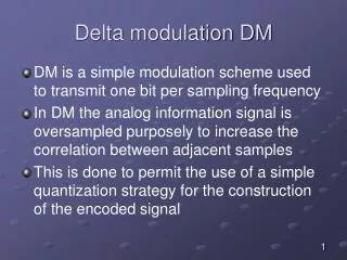
Definition: Delta Modulation is a technique which provides a staircase approximation to an over-sampled version of the message signal (analog input). sampling is at a rate higher than the Nyquist rate – aims at increasing the correlation between adjacent samples; simplifies quantizing of the encoded signal 3.12 Delta Modulation Digital Communication Systems 2012 R.Sokullu
Illustration of the delta modulation process Figure 3.22 Digital Communication Systems 2012 R.Sokullu
message signal is over-sampled difference between the input and the approximation is quantized in two levels - +/-Δ these levels correspond to positive/negative differences provided signal does not change very rapidly the approximation remains within +/-Δ Principle Operation Digital Communication Systems 2012 R.Sokullu
We assume that: m(t) denotes the input message signal mq(t) denotes the staircase approximation m[n] = m(nTs), n = +/-1, +/-2 … denotes a sample of the signal m(t) at time t=nTs, where TS is the sampling period then Assumptions and model Digital Communication Systems 2012 R.Sokullu
we can express the basic principles of the delta modulation in a mathematical form as follow: error signal quantized error signal quantized output Digital Communication Systems 2012 R.Sokullu
Main advantage – simplicity Sampled version of the message is applied to a modulator (comparator, quantizer, accumulator) delay in accumulator is “unit delay” = one sample period (z-1) Pros and cons Digital Communication Systems 2012 R.Sokullu
Figure 3.23DM system. (a) Transmitter. (b) Receiver. Digital Communication Systems 2012 R.Sokullu
Transmitter Side • comparator – computes difference between input signal and one interval delayed version of it • quantizer – includes a hard-limiter with an input-output relation a scaled version of the signum function • accumulator – produces the approximation mq[n] (final result) at each step by adding either +Δ or –Δ • = tracking input samples by one step at a time Digital Communication Systems 2012 R.Sokullu
decoder – creates the sequence of positive or negative pulses accumulator – creates the staircase approximation mq[n] similar to tx side out-of-band noise is cut off by low-pass filter (bandwidth equal to original message bandwidth) Receiver Side Digital Communication Systems 2012 R.Sokullu
slope overhead distortion granular noise Noise in Delta Modulation Systems Digital Communication Systems 2012 R.Sokullu
Slope Overhead Distortion • The quantized message signal can be represented as: • where the input to the quantizer can be represented as: Sample of m(T) at time nT Quantizer input at time (n-1)T So, (except for the quantization error) the quantizer input is the first backward difference (derivative) of the input signal = inverse of the digital integration process Digital Communication Systems 2012 R.Sokullu
Discussion • Consider the max slope of the input signal m(t) • To increase the samples {mq[n]} as fast as the input signal in its max slope region the following condition should be fulfilled: otherwise the step-size Δ is too small Digital Communication Systems 2012 R.Sokullu
In contrast to slope overhead Occurs when step size is too large Usually relatively flat segment of the signal Analogous to quantization noise in PCM systems Granular Noise Digital Communication Systems 2012 R.Sokullu
1. Large step-size is necessary to accommodate a wide dynamic range 2. Small step-size is required for accuracy with low-level signals = compromise between slope overhead and granular noise = adaptive delta modulation, where the step size is made to vary with the input signal (3.16) Conclusion: Digital Communication Systems 2012 R.Sokullu
3.12 Delta Modulation Delta Sigma Modulation 3.13 Linear Prediction 3.14 Differential Pulse Code Modulation 3.15 Adaptive Differential Pulse Code Modulation Outline Digital Communication Systems 2012 R.Sokullu
Conventional delta modulation - Quantizer input is an approximation of the derivative of the input message signal m(t). Results in the accumulation of error (noise) accumulated noise (transmission disturbances) at the receiver (cumulative error). Possible solution: integrating the message before delta modulation – called delta sigma modulation Delta Sigma Modulation Digital Communication Systems 2012 R.Sokullu
The message signal is defined in its continuous form – so pulse modulator contains a hard limiter and a pulse generator to produce a 1-bit encoded signal integration at the tx requires differentiation at the rx side. But: As in conventional DM the message has to be integrated at the final stage this eliminates the need of differentiation here. Remark 1: Digital Communication Systems 2012 R.Sokullu
Block diagrams of systems for realizing Delta-Sigma Modulation Figure 3.25 Digital Communication Systems 2012 R.Sokullu
Integration is a linear operation Int 1 and Int 2 can be combined in a single integrator placed after the comparator (previous slide – 3.25 b) Results in a simpler version of DSM scheme Remark 2: Digital Communication Systems 2012 R.Sokullu
Simplicity of implementation both at the tx and rx side Requires sampling rate far in excess of the Nyquist rate (PCM) – increase in transmission and channel bandwidth If bandwidth is at a premium we have to choose increased system complexity (additional signal processing) to achieve reduced bandwidth. Pros and cons for DSM Digital Communication Systems 2012 R.Sokullu
Reading assignment: 3.13 Linear Prediction (plus all that you are taught in the Signals and Systems – part II) How does it work? Digital Communication Systems 2012 R.Sokullu
3.12 Delta Modulation Delta Sigma Modulation 3.13 Linear Prediction 3.14 Differential Pulse Code Modulation 3.15 Adaptive Differential Pulse Code Modulation Outline Digital Communication Systems 2012 R.Sokullu
Sampling at higher then Nyquist rate creates correlation between samples (good and bad) Difference between samples has small variance – smaller than the variance of the signal itself Encoded signal contains redundant information Can be used to a positive end – remove redundancy before encoding to get a more efficient signal to be transmitted 3.14 Differential PCM Digital Communication Systems 2012 R.Sokullu
How it works – the background • We know the signal up to a certain time • Use prediction to estimate future values • Signal sampled at fs= 1/Ts; sampled sequence – {m[n]}, where samples are Ts seconds apart • Input signal to the quantizer – difference between the unquantized input signal m(t) and its prediction: prediction of the input sample Digital Communication Systems 2012 R.Sokullu
Predicted value – achieved by linear prediction filter whose input is the quantized version of the input sample m[n]. The difference e[n] is the prediction error (what we expect and what actually happens) By encoding the quantizer output we actually create a variation of PCM called differential PCM (DPCM). Digital Communication Systems 2012 R.Sokullu
Figure 3.28DPCM system. (a) Transmitter. (b) Receiver. Digital Communication Systems 2012 R.Sokullu
Details: • Block scheme is very similar to DM • quantizer input • quantizer output may be expressed as: • prediction filter output may be expressed as: Digital Communication Systems 2012 R.Sokullu
If we substitute 3.75 into 3.76 we get: sum is equal to input sample Quantized input of the prediction filter - Digital Communication Systems 2012 R.Sokullu
mq[n] is the quantized version of the input sample m[n] so, irrespective of the properties of the prediction filter the quantized sample mq[n] at the prediction filter input differs from the original sample m[n] with the quantization error q[n]. If the prediction filter is good, the variance of the predictionerrore[n]will be smaller than the variance ofm[n] This means that if we make a very good prediction filter (adjust the number of levels) it will be possible to produce a quantization error with a smaller variance than if the input sample m[n] is quantized directly as in standard PCM Details – cont’d Digital Communication Systems 2012 R.Sokullu
decoder – constructs the quantized error signal quantized version of the input is recovered by using the same prediction filter as at the tx if there is no channel noise – encoded input to the decoder is identical to the transmitter output then the receiver output will be equal to mq[n] (differs from m[n] by q[n] caused by quantizing the prediction error e[n]) Receiver side Digital Communication Systems 2012 R.Sokullu
DPCM and DM DPCM includes DM as a special case Similarities subject to slope-overhead and quantization error Differences DM uses a 1-bit quantizer DM uses a single delay element (zero prediction order) DPCM and PCM both DM and DPCM use feedback while PCM does not all subject to quantization error Comparison Digital Communication Systems 2012 R.Sokullu
Processing Gain • Output signal-to-noise ratio (SNRO) • σM2 – variance of m[n] • σQ2 – variance of quantization error q[n] • rewrite using variance of the prediction error σE2 processing gain signal-to-quanti-zation noise ratio Digital Communication Systems 2012 R.Sokullu
The processing gain Gp when greater than unity represents the signal-to-noise ratio that is due to the differential quantization scheme. For a given input message signal σM is fixed, so the smaller the σE the greater the Gp. This is the design objective of the prediction filter For voice signals – optimal main advantage of DPCM over PCM is b/n 4-11 dB Advantage expressed in terms of bit rate (bits) 1 bit =6 dB of quantization noise (Table 3.35, p 198) So for fixed SNR, sampling rate 8 kHz – DCPM provides saving of 8-16 kb/s (1 -2 bits per sample) PCM Digital Communication Systems 2012 R.Sokullu
3.12 Delta Modulation Delta Sigma Modulation 3.13 Linear Prediction 3.14 Differential Pulse Code Modulation 3.15 Adaptive Differential Pulse Code Modulation Outline Digital Communication Systems 2012 R.Sokullu
PCM for speech coding of 64 kb/s requires high channel bandwidth some applications (secure transmission over radio channel – low capacity) requires speech coding at low bit rates but preserving acceptable fidelity (not 64 kb/s PCM but 32, 16, 8 etc) possible using special coders that utilize statistical characteristics of speech signals and properties of hearing 3.15 Adaptive Differential PCM Digital Communication Systems 2012 R.Sokullu
1. Remove redundancies from speech signals 2. Assign available bits to encode non-redundant parts of speech signal in an efficient way Standard PCM is at 64 kb/s – can be reduced to 32, 16, 8 or even 4 kb/s Price = proportionally increased complexity For same speech quality but Half the bit rate - Computational complexity is an order of magnitude higher Design Objectives Digital Communication Systems 2012 R.Sokullu
ADPCM principles • Allows encoding of speech at 32 kb/s – requires 4 bits per sample • Uses adaptive quantization and adaptive prediction • adaptive quantization – uses a time-varying step Δ[n]. The step-size is varied to match the input signal σM2 • φ is a constant; the other – estimate of the standard deviation - has to be computed continuously Digital Communication Systems 2012 R.Sokullu
Two possibilities: adaptive quantization with forward estimation (AQF) – uses unquantized samples of the input signal to derive forward estimates of σM[n]; requires a buffer to store samples for a certain learning period; incurs delay (~ 16 ms for speech) adaptive quantization with backward estimation (AQB) – uses samples of the quantizer output to derive backwards estimates of σM[n] Digital Communication Systems 2012 R.Sokullu
Adaptive prediction in ADPCM adaptive prediction with forward estimation (APF); uses unqunatized samples of the input signal to calculate prediction coefficients; disadvantages similar to AQF adaptive prediction with backward estimation (APB); uses samples of the quantizer output and the prediction error to compute predictor coefficients; logic for adaptive prediction – algorithm for updating predictor coefficients Digital Communication Systems 2012 R.Sokullu
Figure 3.29 Adaptive quantization with backward estimation (AQB). Digital Communication Systems 2012 R.Sokullu
Adaptive prediction with backward estimation (APB). Figure 3.30 Digital Communication Systems 2012 R.Sokullu
PCM at 64 kb/s and ADPCM at 32 kb/s are internationally accepted standards for voice coding and decoding. Conclusion: Digital Communication Systems 2012 R.Sokullu