Download
1 / 70
760 likes | 5.44k Views
Service Capacity Planning & Waiting Lines. Learning Objectives. Identify or Define: The assumptions of the two basic waiting-line models. Explain or be able to use: How to apply waiting-line models? How to conduct an economic analysis of queues?.

E N D
Service Capacity Planning & Waiting Lines
Learning Objectives • Identify or Define: The assumptions of the two basic waiting-line models. • Explain or be able to use: How to apply waiting-line models? How to conduct an economic analysis of queues?
Elements of Waiting Line Analysis • Elements of a waiting line: arrivals, servers, waiting line. • The Calling Population: Source of customers. • Infinite: Assumes a large number of potential customers, e.g. grocery store, bank etc. • Finite: Has a specific, countable number of potential customers, e.g. repair facility for trucks etc. • The Arrival Rate: Poisson Distribution. • Service Times: Negative Exponential Distribution. • Arrival Rate is less than Service Rate: If not waiting line will continue to grow.
Elements of Waiting Line Analysis • Queue Discipline & Length • Discipline: Order in which customers are served. FCFS, LIFO, Random. • Length: • Infinite: Movie theater. • Finite: bank teller driveway can accommodate only so many cars. • Basic Waiting Line Structures: • Single-Channel, Single-Phase: Post Office with 1-clerk. • Single-Channel, Multiple-Phase: Post Office with more than 1-clerk. • Multiple-Channel, Single-Phase: Nurse-Doctor (Checkup of patients). • Multiple-Channel, Multiple-Phase: Several Nurse-Doctor teams. • Operating Characteristics: • L, Lq, W, Wq, P0, Pn etc. • Describes the performance of the queuing system. • Which the management uses to evaluate the system and make decisions.
Waiting Line Analysis Why is it Important? • Customers regard waiting as a non-value added activity. • Often associated with poor service quality, especially if there is a long wait. • Even in organizations, having employees or work wait is a non-value added activity. • Is a cost to the customers (Customer waiting cost). • Costs the company either to minimize or eliminate waiting OR to lose customers.
Waiting Line System • A waiting line system consists of two components: • The customer population (people or objects to be processed). • The process or service system. • Whenever demand exceeds available capacity, a waiting line or queue forms.
Waiting Line Terminology • Finite versus Infinite populations: • Is the number of potential new customers affected by the number of customers already in queue? • Balking • When an arriving customer chooses not to enter a queue because it’s already too long • Reneging • When a customer already in queue gives up and exits without being serviced • Jockeying • When a customer switches back and forth between alternate queues in an effort to reduce waiting time
Why is there waiting? Waiting lines occur naturally because of two reasons: 1. Customers arrive randomly, not at evenly placed times nor at predetermined times 2. Service requirements of the customers are variable. (Think of a bank for example) Both Arrival & Service Times exhibit a high degree of variability. Leads to Temporarily Overloaded System Waiting Line System Idle (No Customers and hence Waiting Line)
Is there a cost of waiting? • Quantifiable costs: • When the customers are internal (e.g employees waiting for making copies), salaries paid to the employees • Cost of the space of waiting (e.g. patient waiting room) • Loss of business (lost profits) • Hard to quantify costs: • Loss of customer goodwill • Loss of social welfare (e.g. patients waiting for hospital beds)
Capacity -Waiting Trade-off • Waiting lines can be reduced by increasing capacity: • More service counters or servers • Adding workers to increase speed • Install faster processing systems COST!
Queuing Analysis • Mathematical analysis of waiting lines • Goal: Minimize Total Cost • Service capacity costs • Customer waiting costs (difficult to quantify) • Work with an acceptable level of waiting & establish capacity to achieve that level of service. • Traditional Approach: Balance the cost of providing a level of service capacity with the cost of customers waiting for service Minimizes Total Cost. • Economic analysis can be done using either BEA or NPV.
Recap • What is a waiting line? • Why is there waiting? • Elements of Waiting Line Analysis. • Why is it important? • Terminology. • Cost of Waiting: • Quantifiable. • Non-Quantifiable.
Characteristics of Waiting Line • The service system is defined by: • The number of waiting lines • The number of servers • The arrangement of servers • The arrival and service patterns • The service priority rules
Arrival and Service Pattern • Arrival rate: • The average number of customers arriving per time period • Modeled using the Poisson distribution • Service time: • The average number of customers that can be serviced during the same period of time • Modeled using the exponential distribution
Modeling the Arrivals Arrival X X X X X X X Inter-arrival Time Unit Time Period Inter-arrival Time = Time between two consecutive arrivals (a random quantity). Number = Number of arrivals in a unit time period (also a random quantity). How to represent this randomness?? Use Common Probability Distributions.
Modeling the Arrivals Determine the arrival rate () = average number of arrivals per unit time period. Represent Number of arrivals with a Poisson probability distribution with rate (). Represent Inter-arrival time with an Exponential probability distribution with mean (1/ ). Poisson Rate Exponential Inter- of Arrivals Arrival Time
Modeling the Service Determine the service rate () = number of customers that can be served per period. Represent Service Time with an Exponential probability distribution with mean (1/). Poisson Service Rate Exponential Service Time
Number of Lines • Waiting lines systems can have single or multiple queues. • Single queues avoid jockeying behavior & all customers are served on a first-come, first-served fashion (perceived fairness is high) • Multiple queues are often used when arriving customers have differing characteristics (e.g.: paying with cash, less than 10 items, etc.) and can be readily segmented
Server • Single server or multiple/ parallel servers providing multiple channels • Arrangement of servers (phases) • Multiple phase systems require customers to visit more than one server • Example of a multi-phase, multi-server system: 1 4 Arrivals Depart C C C C C 2 5 3 6 Phase 1 Phase 2
Four Types of Queuing Systems Single Channel, Single Phase Single Channel, Multiple Phase Multiple Channel, Single Phase Multiple Channel, Multiple Phase
Common Performance Measure • The average number of customers waiting in queue. • The average number of customers in the system (multiphase systems). • The average waiting time in queue. • The average time in the system. • The system utilization rate (% of time servers are busy). • Probability that an arrival will have to wait.
Rates Customers per unit time
Relationship between the two distributions • An Exponential Service Time means that most of the time, the service requirements are of short duration, but there are occasional long ones. Exponential Distribution also means that the probability that a service will be completed in the next instant of time is not dependent on the time at which it entered the system. • Poisson and Negative Exponential Distributions are alternate ways of presenting the same basic information. • If service time is Exponentially distributed, the Service rate will have Poisson distribution. • If customer arrival rate has a Poisson distribution, the inter-arrival time is Exponential. • E.g. If = 12 / hr --------> Average Service Time = 5 minutes. If = 10 / hr --------> Average inter-arrival time = 6 minutes. Poisson and Exponential Distributions can be derived from each-other. For Poisson: Mean = Variance = . For Exponential: Mean = 1 / & Variance = 1/ 2.
Important Remarks • The use of exponential distributions is a convention. (it makes mathematical analysis simpler) • You have to justify these distributions used in the waiting line models. (by collecting data and then checking for a distribution that fits the data, via statistical tests such as goodness of fit test). • Poisson arrivals is realistic but exponential service is not.
Basic (Steady State) Relationships • Utilization: (should be <1) • Average Number in Service: • Average Number in Queue (Lq ): model dependent • Average Number in System : • Average Time Customers Wait in Queue : Wait in System :
Basic (Steady State) Relationships One of the most important relationship in Queuing Theory is called Little’s Law. Little’s Law: Average Inventory (customers here) = Flow rate (arrival rate here) x Cycle time (average waiting time in queue here)
Two Popular Waiting Line Models 1. Model 1: Single Channel 2. Model 3: Multiple Channel • Single phase • Poisson arrivals • Exponential service times • FCFS queue discipline • No limit on the waiting line length
Example • A help desk in the computer lab serves students on a first-come, first served basis. On average, 15 students need help every hour. The help desk can serve an average of 20 students per hour. • Based on this description, we know: • Mu = 20 (exponential distribution) • Lambda = 15 (Poisson distribution)
Average Utilization where M is number of servers
Average Number of Students Waiting in Line
Average Number of Students in the System
Average Time a Student Spends Waiting in the Line
Average Time a Student Spends in the System
Model3 Lqformula is complicated. Use Table 19-4 on page 824-825 in Book OR page 324 in the Course Pack to read the Lq value. Use the basic relationship formulas to calculate other service measures
Max. K customers Extending Model 1 Other measures from the basic formulas by replacing with eff= (1- PK) (Why?)
Limitations of Waiting Line Models • Mathematical analysis becomes very complicated or intractable for more complex waiting lines. Some examples: • Non-Poisson arrivals • Non-exponential service times • Complex customer behavior (e.g. customers switching between lines, or leaving after some time etc) • multiple phase systems Simulation can be useful analysis tool