Download
1 / 16
180 likes | 767 Views
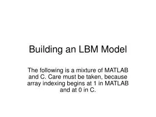
Building an LBM Model. The following is a mixture of MATLAB and C. Care must be taken, because array indexing begins at 1 in MATLAB and at 0 in C. D2Q9 . 6. 2. 5. e 2. e 6. e 5. 0. 3. 1. e 3. e 1. e 4. e 8. e 7. 7. 4. 8. Define velocity vectors.

E N D
Building an LBM Model The following is a mixture of MATLAB and C. Care must be taken, because array indexing begins at 1 in MATLAB and at 0 in C.
D2Q9 6 2 5 e2 e6 e5 0 3 1 e3 e1 e4 e8 e7 7 4 8 Define velocity vectors • In MATLAB, can write ex(0+1)=0, ex(1+1)=1, etc. • %define es • ex(0)= 0; ey(0)= 0 • ex(1)= 1; ey(1)= 0 • ex(2)= 0; ey(2)= 1 • ex(3)=-1; ey(3)= 0 • ex(4)= 0; ey(4)=-1 • ex(5)= 1; ey(5)= 1 • ex(6)=-1; ey(6)= 1 • ex(7)=-1; ey(7)=-1 • ex(8)= 1; ey(8)=-1
Problem definition LY=10 LX=20 tau = 1 g=0.00001 %set solid nodes is_solid_node=zeros(LY,LX) for i=1:LX is_solid_node(1,i)=1 is_solid_node(LY,i)=1 end LY LX % if ~is_interior_solid_node(j,i)
Initialize density and fs (assuming zero velocity) %define initial density and fs rho=ones(LY,LX); f(:,:,1) = (4./9. ).*rho; f(:,:,2) = (1./9. ).*rho; f(:,:,3) = (1./9. ).*rho; f(:,:,4) = (1./9. ).*rho; f(:,:,5) = (1./9. ).*rho; f(:,:,6) = (1./36.).*rho; f(:,:,7) = (1./36.).*rho; f(:,:,8) = (1./36.).*rho; f(:,:,9) = (1./36.).*rho;
// Computing macroscopic density, rho, and velocity, u=(ux,uy). for( j=0; j<LY; j++) { for( i=0; i<LX; i++) { u_x[j][i] = 0.0; u_y[j][i] = 0.0; rho[j][i] = 0.0; if( !is_solid_node[j][i]) { for( a=0; a<9; a++) { rho[j][i] += f[j][i][a]; u_x[j][i] += ex[a]*f[j][i][a]; u_y[j][i] += ey[a]*f[j][i][a]; } u_x[j][i] /= rho[j][i]; u_y[j][i] /= rho[j][i]; } } }
On boundary, ‘neighboring’ point is on opposite boundary Periodic Boundaries ip = ( i<LX-1)?( i+1):( 0 ); in = ( i>0 )?( i-1):( LX-1); jp = ( j<LY-1)?( j+1):( 0 ); jn = ( j>0 )?( j-1):( LY-1); where LHS = (COND)?(TRUE_RHS):(FALSE_RHS); means if( COND) { LHS=TRUE_RHS;} else{ LHS=FALSE_RHS;}
// Compute the equilibrium distribution function, feq. f1=3.; f2=9./2.; f3=3./2.; for( j=0; j<LY; j++) { for( i=0; i<LX; i++) { if( !is_solid_node[j][i]) { rt0 = (4./9. )*rhoij; rt1 = (1./9. )*rhoij; rt2 = (1./36.)*rhoij; ueqxij = uxij; //Can add forcing here; see MATLAB code ueqyij = uyij; uxsq = ueqxij * ueqxij; uysq = ueqyij * ueqyij; uxuy5 = ueqxij + ueqyij; uxuy6 = -ueqxij + ueqyij; uxuy7 = -ueqxij + -ueqyij; uxuy8 = ueqxij + -ueqyij; usq = uxsq + uysq;
feqij[0] = rt0*( 1. - f3*usq); feqij[1] = rt1*( 1. + f1*ueqxij + f2*uxsq - f3*usq); feqij[2] = rt1*( 1. + f1*ueqyij + f2*uysq - f3*usq); feqij[3] = rt1*( 1. - f1*ueqxij + f2*uxsq - f3*usq); feqij[4] = rt1*( 1. - f1*ueqyij + f2*uysq - f3*usq); feqij[5] = rt2*( 1. + f1*uxuy5 + f2*uxuy5*uxuy5 - f3*usq); feqij[6] = rt2*( 1. + f1*uxuy6 + f2*uxuy6*uxuy6 - f3*usq); feqij[7] = rt2*( 1. + f1*uxuy7 + f2*uxuy7*uxuy7 - f3*usq); feqij[8] = rt2*( 1. + f1*uxuy8 + f2*uxuy8*uxuy8 - f3*usq); } } }
Collide // Collision step. for( j=0; j<LY; j++) for( i=0; i<LX; i++) if( !is_solid_node[j][i]) for( a=0; a<9; a++) { fij[a] = fij[a] + ( fij[a] - feqij[a])/tau; }
Bounceback Boundaries • Bounceback boundaries are particularly simple • Played a major role in making LBM popular among modelers interested in simulating fluids in domains characterized by complex geometries such as those found in porous media • Their beauty is that one simply needs to designate a particular node as a solid obstacle and no special programming treatment is required
Collision (solid nodes): Bounceback // Standard bounceback. temp = fij[1]; fij[1] = fij[3]; fij[3] = temp; temp = fij[2]; fij[2] = fij[4]; fij[4] = temp; temp = fij[5]; fij[5] = fij[7]; fij[7] = temp; temp = fij[6]; fij[6] = fij[8]; fij[8] = temp;
// Streaming step. for( j=0; j<LY; j++) { jn = (j>0 )?(j-1):(LY-1) jp = (j<LY-1)?(j+1):(0 ) for( i=0; i<LX; i++) { if( !is_interior_solid_node[j][i]) { in = (i>0 )?(i-1):(LX-1) ip = (i<LX-1)?(i+1):(0 ) ftemp[j ][i ][0] = f[j][i][0]; ftemp[j ][ip][1] = f[j][i][1]; ftemp[jp][i ][2] = f[j][i][2]; ftemp[j ][in][3] = f[j][i][3]; ftemp[jn][i ][4] = f[j][i][4]; ftemp[jp][ip][5] = f[j][i][5]; ftemp[jp][in][6] = f[j][i][6]; ftemp[jn][in][7] = f[j][i][7]; ftemp[jn][ip][8] = f[j][i][8]; } } }
Incorporating Forcing (gravity) • Gravitational acceleration is incorporated in a velocity term ueqxij = u_x(j,i)+tau*g; %add forcing