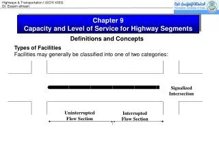
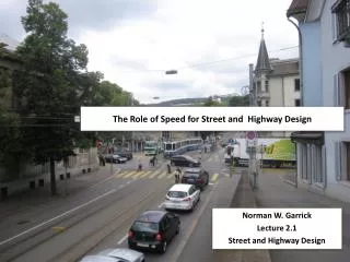
Interpreting Demand and Capacity for Street and Highway Design

1. Interpreting Demand and Capacity for Street and Highway Design Lecture 5.1 CE 4720 5720 Norman Garrick Norman W. Garrick

2. Travel Flow Data Some Basic Concepts Good travel flow data for all modes of travel is important for transportation design. One of the challenges is that travel flow varies significantly in both space and time. We often do not have data at a fine enough resolution to fully capture these variations. It is important to understand the likely variations in order to effectively interpreter the available data Norman W. Garrick

3. Temporal Variation in Traffic Flow Monday to Thursday Saturday Traffic flow vary by time of day, day of week, month of year and from year to year. The pattern of variation depends on the specific location. For example, the temporal variation of traffic in Storrs is likely to be different from that in Willimantic. http://www.ptt.uni-duisburg.de/en/projekte/babnrw/daten/ Norman W. Garrick

4. Temporal Variation in Traffic Flow One solution that is some times used to reduce temporal variation is differential pricing. For example, many transit systems charge a higher rate for travel before 10 am and after 3 pm. This helps encourage people that have flexible plans to delay their travel to the off peak time. This is the same approach used on some toll roads where the plan is know as congestion pricing. Norman W. Garrick

5. Spatial Variation in Traffic Flow http://www.interstate-guide.com/images/i-077_va_aadt.gif Norman W. Garrick

6. Spatial Variation in Traffic Route 195 - Storrs Storrs Mile Zero Willimantic Norman W. Garrick

7. Spatial Variation in Traffic Volume on Route 195, Storrs2006 ADT by Mileage East Brook Mall/Big Y UConn/Storrs Center Norman W. Garrick

8. Directional in Traffic FlowDirectional Variation Reversible lanes in the middle to deal with a severe directional variation. (I believe this is just conceptual – I don’t know of any example of reversible lanes implemented in this manner. Norman W. Garrick

9. Directional in Traffic FlowThe Zipper Machine Norman W. Garrick

10. Directional Distribution In many urban areas trips are mostly going towards the central business district in the morning and from the CBD in the evening. This means that the trains and the roads are sized to carry the peak direction flow. If the directional distribution is very lopsided then this is a very inefficient system since the lanes and the trains going away from the center will be virtually empty in the morning. One argument for mixed land use is that it helps to cut down on this directional over balance. So if a train is connect two mixed use centers (such as downtown DC and Arlington, Virginia) the directional distribution will be more balanced resulting in more efficient use of the transportation system. Norman W. Garrick

11. Where does travel flow counts come from? State Counts of Vehicle Traffic The DOT maintain a program for counting traffic on all state owned highways, roads and streets. There are two different type of counts: permanent count stations and temporary count stations Permanent Count Stations give the most complete coverage of temporal variation in traffic Temporary count stations are much less reliable since they are put out for at most 48 hours – the state then use factors to estimate the average daily count. Other source of traffic count data are counts from individual towns or from developers working on larger projects. Norman W. Garrick

12. Where does travel flow counts come from? Pedestrian, Bikes and Transit Counts I know of no agencies that routinely count pedestrian traffic – this makes it harder to include pedestrian issues in transportation planning A handful of cities in the country, including Portland, Davis and Cambridge have programs for counting bike traffic Transit counts are readily available from transit agencies and national transit bodies Norman W. Garrick

13. Cyclists per Day Bikeway Miles 1991 2007 Portland (OR) Bike Count Program http://www.streetsblog.org/wp-content/uploads/2007/09/portland_bike_counts.jpg

14. Shared Bikes, ParisA New Era for Bike Countshttp://networkedblogs.com/g0g87(from Sam Goater) Norman W. Garrick

15. Bike Parking at Train Station, Amsterdam Norman W. Garrick

16. What is the State Traffic Counts Used for?AADT The state traffic count is used to estimate an average annual daily traffic (AADT) The AADT is meant to represent the average traffic over all 365 days in the year. In other words, it is meant to be Total Traffic in year / 365 This can be obtained relatively accurately from the permanent count stations. From the temporary stations, this is more difficult. The count from the station (which is referred to as average daily traffic or ADT) is multiplied by seasonal and day of the week adjustment factor to get an estimated AADT. Norman W. Garrick

17. Characterizing Traffic Counts Vehicles/hr or AADT Often reports from state level traffic count studies give average annual daily traffic (AADT) Since hourly volume for the design hour is what is typically used for design it is left up to the designer to come up with a reasonable design hourly volume from the AADT As a very rough guide the typical design hour volume is can be taken as about 10% of the AADT. But this % varies significantly depending on the temporal variation in traffic. Once a design hour volume is determined then the designer must also determine the directional split. Norman W. Garrick

18. ADT and Design Hour Volume – Rural Roads Norman W. Garrick

19. Demand and Capacity for Street and Highway Design Convention street and highway design is based on the idea of fitting capacity to demand Demand is characterized by a design hour volume Capacity is characterized by design hourly service volume Norman W. Garrick

20. Demand The design hour volume is meant to be the volume of traffic that will use the facility in the design hour, in the design direction, in the design year Usually the design hour is taken as the 30 busiest hour of the year DHV is often estimated from AADT Norman W. Garrick

21. Estimating Traffic in the Design Year In many projects, the DHV is based on traffic for 20 or 30 years in the future The procedure for doing this is some times derided as ‘predict and provide’ because in many cases it is based just on predicting past trends Norman W. Garrick

22. Problems with Predict and Provide Predict and provide is problematic because expanding capacity affects future demand. Providing increase capacity lead to more traffic volumes in the future than we would otherwise have. Over the last 60 years this has lead to a self re-enforcing cycle of increasing traffic. But, recent trends suggest that this cycle might be at an end. Norman W. Garrick

23. Traffic Trends in USA Norman W. Garrick

24. Traffic Trends in ConnecticutRoute 195 Data Norman W. Garrick

25. Predict and Provide in an Era of Decreasing Traffic Decreasing or steady traffic volumes is one more reason to reject the concept of predict and provide Basing design decisions on a 20 or 30 year prediction of traffic volume is increasingly unacceptable Norman W. Garrick

26. CapacityHow is the capacity of the Hoover Dam Determined? Norman W. Garrick

27. What is the Capacity of a Street? Norman W. Garrick

28. What is the Capacity of a Street? Norman W. Garrick

29. Understanding Capacity for Vehicle Travel The designer has flexibility in selecting a design capacity She does this by designating a Level of Service Once a LOS is determined then the design hourly service volume can be selected from a chart Determining vehicle capacity on a street is not really like determining the amount of water in a measuring jar Capacity is not a fixed number – it is rather a number selected based on what level of congestion we are willing to put up with Norman W. Garrick

30. LOS for FreewaysLOS in urban areas is usually based on intersection flow Norman W. Garrick

31. Capacity and the Level of Service What are the trade-offs involved in selecting a low LOS? Norman W. Garrick

32. Capacity and the Level of Service Some cities now require that we design for LOS E or F to reduce inefficiency and the impact on the urban area of having large facilities Selecting a low LOS means that you are designing for a low level of congestion during the busiest hour of the year That means the facility will be empty for most hours in the day Norman W. Garrick

33. New View of Street Capacity In the past, Street Capacity = Design Hour Service Volume Now, Street Capacity = Social Capacity + Economic Capacity + Travel Capacity By Ian Lockwood Norman W. Garrick

34. Sample Calculation 1

35. LOS, Volume CapacitySample Calculation A two lane urban street has an ADT of 20,000 vehicles per day. Estimate what fraction of the year this street will operate at i) LOS E, ii) LOS D. Do this calculation for directional splits of 50% and 60%. The hourly volume distribution and the design hour service volumes are given on the following sheets.

36. Traffic Hourly Distribution Hour volume as % of ADT Number of Hours with traffic great than shown

37. Design Hour Service Volume Urban Streets with Frequent Signal Controlled Intersections Source: http://www.dot.state.fl.us/planning/systems/sm/los/pdfs/lostables.pdf Assumptions: > 4.5 Signalized intersection, 1.5 % heavy traffic, 12 % left turn, 12 % right turn

38. Sample Calculations 2

40. Ocean Springs – Biloxi Bridge

41. Biloxi – Gulfport Region

42. Ocean Springs – Biloxi Bridge Location

43. Ocean Springs – Biloxi BridgeADT Pre-Construction

44. Design Hour Service Volume Source: AASHTO 1990

45. LOS, Volume CapacityOcean Springs – Biloxi Bridge Estimate the level of service for the Ocean Springs – Biloxi Bridge.

46. Why is this Road So Empty? • Predict and provide for 30 year in future • Design for 30th busiest hour of year • Design using a capacity based on low LOS