Download

1 / 52
530 likes | 551 Views
Newsvendor Models & the Sport Obermeyer Case. John H. Vande Vate Spring, 2012. Issues. Learning Objectives: We’ve discussed how to measure demand uncertainty based on historical forecast accuracy How to accommodate uncertainty in sourcing

E N D
Newsvendor Models & the Sport Obermeyer Case John H. Vande Vate Spring, 2012 1
Issues • Learning Objectives: • We’ve discussed how to measure demand uncertainty based on historical forecast accuracy • How to accommodate uncertainty in sourcing • Low cost, high commitment, low flexibility (“contract”) • Higher cost, low commitment, higher flexibility (“spot”) 2
Finding the Right Mix • Managing uncertainty • Low cost, high commitment, low flexibility (“contract”) • Higher cost, low commitment, higher flexibility (“spot”) 3
More Generally • Contracts with Carriers • Assured capacity via contracts • Meet volatile demand with spot • Labor • Full-time employees • Over-time • Temporary workers • Capacity • Internal “owned” • Outsourced • Inventory • Safety Lead Time • Expedited Shipments 4
Obermeyer’s Challenge • Long lead times: • It’s November ’92 and the company is starting to make firm commitments for it’s ‘93 – 94 season. • Little or no feedback from market • First real signal at Vegas trade show in March • Inaccurate forecasts • Deep discounts • Lost sales 5
Production Options • Hong Kong • More expensive • Smaller lot sizes • Faster • More flexible • Mainland (Guangdong, Lo Village) • Cheaper • Larger lot sizes • Slower • Less flexible 6
The Product • 5 “Genders” • Price • Type of skier • Fashion quotient • Example (Adult man) • Fred (conservative, basic) • Rex (rich, latest fabrics and technologies) • Beige (hard core mountaineer, no-nonsense) • Klausie (showy, latest fashions) 7
The Product • Gender • Styles • Colors • Sizes • Total Number of SKU’s: ~800 8
Service • Deliver matching collections simultaneously • Deliver early in the season 9
Production Planning Example • Rococo Parka • Wholesale price $112.50 • Average profit 24%*112.50 = $27 • Cost = 76%*112.50 = $85.50 • Average loss (Cost – Salvage) • 8%*112.50 = $9 • Salvage = (1-24%-8%)*112.50 • = (1-32%)*112.50 • = 68%*112.50 • = $76.50 10
Sample Problem Forecast is average of the “experts” forecasts Std dev of demand about forecast is 2x std dev of forecasts Why 2? It has worked 11
Our Approach • Keep records of Forecast and Actual sales • Construct a distribution of ratios Actual/Forecast • Assume next ratio will be a sample from this distribution 12
Distribution of Demand • We have an estimated distribution of demand (however we get it) • Example Gail • Mean 1,017 units • Standard deviation 388 units • Question: How many items to order? 13
Margin %* Price (1-Margin %)* Price*Order Qty ObermeyerData.xls (1-Margin %-Loss %)* Price Incr. Rev./Cost Min(Order Qty, Actual Demand)* Price Revenue + Salvage - Cost Max(0, Order Qty-Actual Demand)* Salvage Value 14
What’s the Right Answer? • There is no “right” order quantity, we don’t know what demand will be • What’s the right approach to choosing an answer? 15
Meaningful Objective • Maximize the Expected Profit? 16
Marginal ROIC • Marginal Return on Investment: • Questions: • What happens to Marginal Expected Profit per unit as the order quantity increases? • What happens to the Marginal Invested Capital as the order quantity increases? • What happens to Marginal Return on Investment as the order quantity increases? • What order Quantity maximizes Marginal Return on Investment? • Which styles will show the higher Marginal Return on Investment? Marginal Expected Profit Marginal Invested Capital 17
Basics: Selecting an Order Quantity • News Vendor Problem • Order Q • Look at last item, what does it do for us? • Increases our (gross) profits (if we sell it) • Increases our losses (if we don’t sell it) • Expected impact? • Gross Profit*Chances we sell last item • Loss*Chances we don’t sell last item • Expected impact • P = Probability Demand < Q, the Cycle Service Level • (Selling Price – Cost)*(1-P) • (Cost – Salvage)*P Expected reward: Why 1-P? Expected risk: Why P? 18
Question • Expected impact • P = Probability Demand < Q • Reward: (Selling Price – Cost)*(1-P) • Risk: (Cost – Salvage)*P • How much to order? 19
How Much to Order • Balance the Risks and Rewards Reward: (Selling Price – Cost)*(1-P) Risk: (Cost – Salvage)*P (Selling Price – Cost)*(1-P) =(Cost – Salvage)*P P = If Salvage Value is > Cost? 20
How Much to Order • For Gail: P = Selling Price – Cost = 24%Price Selling Price – Salvage = Selling Price – Cost + Cost – Salvage = 24% Price + 8%Price = 32% Price P = 24/32 = 75% What does this mean? 21
For Obermeyer • Ignoring all other constraints recommended target Stock Out probability is: = 8%/(24%+8%) = 25% We’ll use 8% of wholesale and 24% of wholesale across all products 22
Simplify our discussion • Every product has • Gross Profit = 24% of wholesale price • Cost – Salvage = 8% of wholesale price • Use Normal distribution for demand • Mean is the average forecast • Std dev is 2X the std. dev. of the forecasts • Every product has recommended P = 0.75 • What does this mean? 23
Ignoring Constraints Everyone has a 25% chance of stockout Everyone orders Mean + 0.6745s P = .75 [from .24/(.24+.08)] Probability of being less than Mean + 0.6745s is 0.75 24
Does this make sense? Why not do this? 25
P = 0.75 • Explain the strategy • Which products are riskier? • Which are safer? 26
Constraints • Make at least 10,000 units in initial phase • Minimum Order Quantities • What issues should we consider in choosing what to make in the initial phase? • What objective to consider when choosing what to make in the initial phase? 27
Invested Capital • The landed cost (to get product to Obermeyer) is the “investment” • We’ll assume Invested Capital is Cost • Cost = (1-24%)*Price = 76% Price 28
Objective for the “first 10K” • Invest first in those items with the highest marginal return • Questions: • What happens to Marginal Expected Profit per unit as the order quantity increases? • What happens to the Marginal Invested Capital per unit as the order quantity increases? • What happens to Marginal Return on Investment as the order quantity increases? • Which styles will show the higher Marginal Return on Investment? Marginal Expected Profit Marginal Invested Capital 29
Alternative Approach • Maximize Expected Profits over the season by simultaneously deciding early and late order quantities • See Fisher and Raman Operations Research 1996 • Requires us to estimate before the Vegas show what our forecasts will be after the show. 30
First Phase • Allocate the next units to the SKU with the highest marginal ROIC • Stop when we’ve allocated all 10,000 units 31
First Phase Objective: • ci is the invested capital (cost) per unit • For a given MROIC • Max Expected Profit – MROIC SciQi • The objective is separable • Max Expected Profit(Qi)-MROIC*ciQi • Set derivative to 0 • Marginal Expected Profit- MROIC*ci = 0 • MROIC = Marginal Expected Profit Marginal Invested Capital 32
First Phase Objective: • We find Qi so that • Marginal Expected Profit- MROIC*ci = 0 • = MROIC • What does this mean about each unit we order? Marginal Expected Profit(Qi) Marginal Invested Capital 33
Solving • Adjust MROIC until SQi = 10,000 • Why =? • How to accomplish this? 34
Ordering • As though we • Sorted the units of the different skus in decreasing order of marginal ROIC • Took the top 10,000 35
Solving for Qi • For MROIC fixed, how to solve Maximize S Expected Profit(Qi) - MROIC S ciQi s.t. Qi 0 • Remember it is separable (separate decision for each item) • Exactly the same thinking as the News Vendor • Last item: • Reward: Profit*Probability Demand exceeds Q • Risk: (Cost – Salvage)* Probability Demand falls below Q • MROIC? • MROIC is like a tax or interest on the investment that adds MROIC * ci to the cost. We pay it whether the item sells or not. • If it sells, get the original profit – MROIC* ci • If it doesn’t sell, get (Salvage – Cost – MROIC*ci) 36
Solving for Qi • Last item: • Reward: • (Revenue – Cost – MROIC*ci)*Prob. Demand exceeds Q • (Revenue – Cost – MROIC*ci)*(1-P) • Risk: • (Cost + MROIC*ci – Salvage) * Prob. Demand falls below Q • (Cost + MROIC*ci – Salvage) * P • As though Cost increased by MROIC*ci , the “Tax” or “Interest” we pay to investors 37
Hong Kong: Solving for Qi • Balance the two (Revenue – Cost – MROIC*ci)*(1-P) = (Cost + MROIC*ci – Salvage)*P • So P = (Profit – MROIC*ci)/(Revenue - Salvage) • P = Profit/(Revenue - Salvage) – MROIC*ci/(Revenue - Salvage) • What happens to P as MROIC increases? • What happens to Qi as MROIC increases? 38
Summary • Hong Kong • Cost = 76% of Wholesale price • Profit = 24% of Wholesale price • Salvage Value = 68% of Wholesale price • If we don’t sell an item, we lose our investment of 76% of wholesale price, but recoup 68% in salvage value. So, net we lose 8% of wholesale price 39
Hong Kong: Solving for Qi • So P = (Profit – ROIC*ci)/(Revenue - Salvage) • = Profit/(Revenue - Salvage) – ROIC*ci/(Revenue - Salvage) • In our case • (Revenue - Salvage) = 32% Revenue, • Profit = 24% Revenue • ci = 76% Revenue So P = 0.75 – MROIC*76%/32% = 0.75 – 2.375*MROIC 40
Q as a function of MROIC Q ROIC 41
Let’s Try It Min Order Quantities! 42
Summary • China • Cost = 68.75% of Wholesale price • Profit = 31.25% of Wholesale price • Salvage Value = 68% of Wholesale price • If we don’t sell an item, we lose our investment of 68.75% of wholesale price, but recoup 68% in salvage value. So, net we lose 0.75% of wholesale price 43
In China: Solving for Q • So P = (Profit – MROIC*ci)/(Revenue - Salvage) = Profit/(Revenue - Salvage) – MROIC*ci/(Revenue - Salvage) • In our case • (Revenue - Salvage) = 32% Revenue, • Profit = 31.25% Revenue • ci = 68.75% Revenue So P = 31.25/32 – MROIC*68.75%/32% = 0.977 – 2.148*MROIC 44
38.73% vs 25.5% And China? Min Order Quantities! Why the same? 45
And Minimum Order Quantities In Hong Kong: As we drive up the MROIC, what’s happening to Qi? When Qi reaches 600 (the lower bound), what do we know about Marginal Expected Profit Marginal Investment What should happen to Qi for values of MROIC higher than this? 46
If everything is made in one place, where would you make it? Answers Hong Kong China 47
Summary • Simple question of how much to make (no minimums, no issues of before or after the Vegas show) • Maximize expected profit • That’s just a newsvendor problem • Trade off risk of lost sales vs risk of salvage • Decide which 10,000 to make before show (no minimums, no choice of where to make them) • Highest marginal return on invested capital 48
Summary • Impose minimums (no choice of where to make them) • If the tax rate exceeds the MROIC at the minimum order quantity, don’t make the product. Otherwise, make at least the minimum order quantity • Where to make the product? • China • Hong Kong 49
Where to Produce? 1 if We don’t make the product in China and MROIC is < Marginal Return at 600 If a style is not attractive to produce in China, it might be attractive in HK at the lower MOQ… 50