Download

1 / 25
250 likes | 271 Views
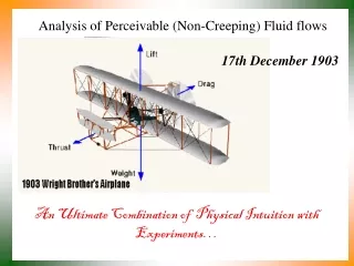
Analysis of Creeping Flows. P M V Subbarao Professor Mechanical Engineering Department I I T Delhi. Highly Viscous Flows…. "Every high-school student learns that Millikan calculated the drag of an oil drop using the approximation developed by Stokes in 1851".

E N D
Analysis of Creeping Flows P M V Subbarao Professor Mechanical Engineering Department I I T Delhi Highly Viscous Flows….
"Every high-school student learns that Millikan calculated the drag of an oil drop using the approximation developed by Stokes in 1851" That gave to Robert Millikan Nobel prize in 1923.
Importance of Creeping Flows in 21st Century • Small Reynolds flows receive a new impulse nowadays. There is a huge interest in "microhydrodynamics. • This new interest comes from the fact that lot of applications in biological field. • Flow past • blood cells, • spermatozoids, • swimming microorganisms. • Flows in small devices • MEMS, • lab on chip.... • Stokes flow can be at large scale with slow velocity and high viscosity • in geophysics, flow in porous media, flow of lava or ice.
The Creeping Flow Any viscous flow, whose curl of curl of vorticity is zero is called as stokes flow or creeping flow Consider two-dimensional flows: 2D-Cartesian : 2D-Cylindrical : 2D-Spherical :
Stream Function (Cartesian) Cartesian coordinates, the two-dimensional continuity equation for steady incompressible flows: If we define a stream function, y, such that: Then the two-dimensional continuity equation becomes:
Geometry of Creeping flows Consider Cartesian System: Creeping flow Equations: Introduce Stream function,(x,y).
Symmetry of the Spherical Geometry The flow will be symmetric with respect to .
Cartesian Uniform Velocity in Spherical System Component of incident velocity in the radial direction, Incident Velocity Component of incident velocity in the - direction, Cartesian Uniform velocity in spherical system:
Vorticity of 2-D Flow in Spherical System • The only component of vorticity in this axisymmetric problem is ωϕ, and is given by Strokes defined a stream function in spherical coordinate system (1851) as: The stokes solution to be evaluated is:
Stokes Flow in terms of Stream Function the momentum equation as a scalar equation for ψ.
Flow on the Surface of a Sphere As Predicted by Euler & Bernoulli
Imagination of Flow on the Surface of a Sphere Stokes Imagination : Creeping Flow Euler’s Imagination: Nonviscous Flow Velocity Larger velocity near the sphere is an inertial effect.
General Flow around a Sphere A more general case Incident velocity is approached far from the sphere. Increased velocity as a result of inertia terms. Shear region near the sphere caused by viscosity and no-slip.
Stokes Problem The boundary conditions
Far-field Boundary Conditions in Terms of From definition: which suggests the -dependence of the solution.
Separability Again, at r=R: and at r : For a separable solution, we look for a form: Because the q-dependence holds for all q, but the r-dependence does not, we must write:
Low Re Uniform Flow Past A Sphere Again, at r=R: and at r : For a separable solution, we look for a form:
Method of Separation of variables The problem yields readily to a product solution (r, ) = f(r)g().
The Momentum Equation as ODE f(r) is governed by the equi-dimensional differential equation: whose solutions are of the form f(r) ∝ rn It is easy to verify that n = −1, 1, 2,4 so that
Evaluation of Constants The boundary conditions