Download
1 / 25
250 likes | 421 Views
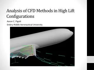
Understanding the Shortcomings of CFD in Predicting High Lift Configurations. Ciara Thompson Embry- Riddle Aeronautical University. Purpose. Background 2 nd AIAA High Lift Prediction Workshop Assess the prediction capabilities of current CFD Technology

E N D
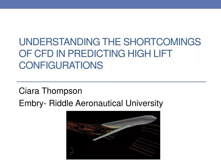
Understanding the Shortcomings of CFD in Predicting High Lift Configurations Ciara Thompson Embry- Riddle Aeronautical University
Purpose • Background • 2nd AIAA High Lift Prediction Workshop • Assess the prediction capabilities of current CFD Technology • Validate CFD results by comparing to wind tunnel experiments • Compare CFD surface flow images to wind tunnel oil flow visualization images • Overview • Experiment • CFD • Experimental and CFD Data Comparison • Discussion • Further Work • Acknowledgments • Q &A
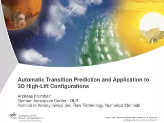
Model • KH3Y geometry • DLR-F11 model • EUROLIFT Project
Experiment • Conditions • Low speed wind tunnel test with an operating range of 60m/s • Reynolds number 1.35e6 • Mach number of 0.175 • DataAnalyzed • Oil flow visualization
CFD • Cray XE6 • 1024 compute cores • 24 hours of wall-clock time to converge • 7GB per file • OVERFLOW 2.2e • Reynolds-Averaged Navier-Stokes solver by Pieter Buning, NASA Langley • Structured Cartesian grid-69 million grid points • Solver settings • Spalart-Allmaras • AOA-7,18.5 and 21 degrees • 1 equation turbulence model http://www.cray.com
CFD Post Processing Procedure • Processed Data Provided by Dr. Earl P.N. Duque • Computing Power • 6 core AMD PhenomΙΙProcessor • 16GB memory • FieldView 14 • Created surface streamlines using surface flow tool • CFD Surface flow tool mimics oil flow visualization • Challenges • Slow
CFD Post Processing Results • Configuration 2 • Configuration 4 • Configuration 5 α=7̊ α=21̊ α=18.5̊ α=7̊ α=18.5̊ α=21̊ α=21̊ α=7̊ α=18.5̊
8 Experimental and CFD Data Comparison α=7̊ Alpha: 7 degrees Color Code Pink – Separation Green - Surface flow lines Blue Lines- Reattachment Reattachment lines Experiment -Oil Flow Visualization α=7̊ CFD-Streamlines
9 Experimental and CFD Data Comparison CFD α=7̊ Separationlines Experiment α=7̊
10 Experimental and CFD Data Comparison α=18.5̊ Color Code Pink – Separation Green - Surface flow lines Blue Lines- Reattachment Alpha: 18.5 degrees Reattachment lines Separation Bubble Experiment -Oil Flow Visualization α=18.5̊ CFD-Streamlines
11 Experimental and CFD Data Comparison α=21̊ Color Code Pink – Separation Green - Surface flow lines Blue Lines- Reattachment Alpha: 21 degrees Reattachment lines Separation Bubble Experiment -Oil Flow Visualization α=21̊ CFD-Streamlines
Shear Stress: Configuration 5 α=7̊ α=18.5̊ α=21̊
Experimental and CFD Data Comparison CFD • Major Inconsistency α=18.5̊ Experiment α=18.5̊ α=21̊
Experimental and CFD Data Comparison CFD α=21̊ Experiment α=21̊
Discussion • The results showed inconsistency in flow at higher angles of attack • Inconsistency may be a result of • CFD physical models • Wind tunnel errors
Future Work • Compare surface flow of configurations 2,4 and 5 • Compare pressure distribution of configurations 2, 4 and 5 • Determine the causes of inconsistency between experimental data and CFD data
Acknowledgments • CFD images were created using FieldView as provided by Intelligent Light through its University Partners Program • Simulations were performed by Dr. Earl P.N. Duque, Manager of Applied Research, Intelligent Light • NASA Space Grant • Faculty Advisor Dr. Shigeo Hayashibara
References • Rudnik, R., Huber, K., Melber-Wilkending, S. “EUROLIFT Test Case Description for the 2nd High Lift Prediction Workshop”, AIAA 2012-2924, 2012 • Nichols,R., Bunning,P., “User’s Manual for Overflow 2.2”, August 2010 • Intelligent Light, FieldVIew 14, Software Package, Ver. 14, Rutherford, NJ • Christopher, R., “2nd AIAA CFD High Lift Prediction Workshop (HiLiftPW-2)”, NASA [http://hiliftpw.larc.nasa.gov/] All experimental results shown here were obtained from AIAA 2012-2924
CFD- Code • OVERFLOW 2.2e • This code is a finite difference mesh and solver • It is a three dimensional time marching implicit Navier-Stokes code which can also be used for two-dimensional or axisymmetric mode • The mesh is a structured grid system which consists of an overset of Cartesian grids to develop the desired model • The model was meshed with a medium grid
AIAA High Lift Prediction Workshop(Background) • The aim of the High –Lift PW was to assess the prediction capabilities of current CFD technology and to enhance CFD prediction capability for high lift configurations • The 2nd workshop was based on an experiment conducted under the German Aerospace Center for the European project EUROLIFT • The experiment was based on a typical geometry of a commercial high lift aircraft developed for the project and defined as the KH3Y geometry. The model was developed by the German Aerospace Center and denominated as the DLR-F11 • The experiment was conducted in the low speed wind tunnel of Airbus in Bremen, Germany and in the high speed European Transonic Wind tunnel AIAA 2012-2924
Experiment • Model • The experimental model consists of a fuselage, and wing consisting of the following components: leading edge slat, and trailing edge Fowler flap • Two configurations were developed • Landing Configuration • Take off Configuration • The dimensions of the model are as follows http://hiliftpw.larc.nasa.gov/
CFD: Solver Settings • Turbulence model • Spalart-Allmaras • 1 equation turbulence model derived using empirical relationships, dimensional analysis and Galilean invariance • Fast and numerically stable turbulence model suitable of shear layers and boundary layers Mathematical description the turbulence model • The mathematical model describes the production and dissipation of the turbulence