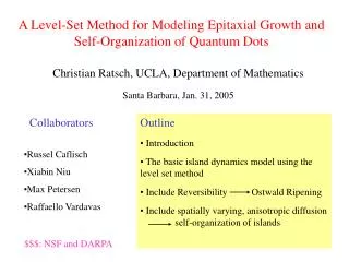
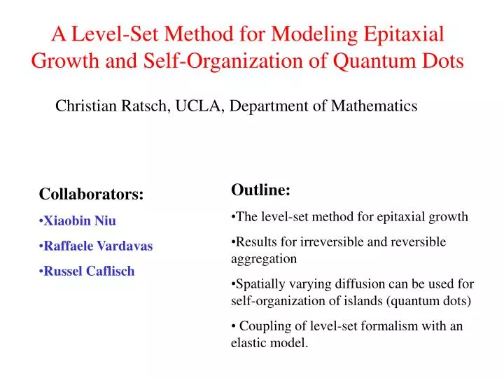
A Level-Set Method for Modeling Epitaxial Growth and Self-Organization of Quantum Dots

1. A Level-Set Method for Modeling Epitaxial Growth and Self-Organization of Quantum Dots Christian Ratsch, UCLA, Department of Mathematics • Outline: • The level-set method for epitaxial growth • Results for irreversible and reversible aggregation • Spatially varying diffusion can be used for self-organization of islands (quantum dots) • Coupling of level-set formalism with an elastic model. • Collaborators: • Xiaobin Niu • Raffaele Vardavas • Russel Caflisch

2. Modeling thin film growth • Methods used • (Atomistic) KMC simulations: • Completely stochastic method • Rate parameters can be obtained from DFT • Continuum equations (PDEs): • essentially deterministic • no microscopic details. • parameters can be obtained from atomistic model (but difficult) • New Method • Level set method: • PDE - based, (almost) deterministic • atomistic details can be included • microscopic parameters can be obtained from DFT

3. Island dynamics Atomistic picture(i.e., kinetic Monte Carlo) F v D • Describe motion of island boundaries by a level-set function • Adatoms are described in a mean-field approach with a diffusion equation Idea of the level set appproach

4. Level set function j Surface morphology j=0 j=0 t j=0 j=1 j=0 The level set method: schematic • Level set function is continuous in plane, but has discrete height resolution • Adatoms are treated in a mean field picture

5. Diffusion equation for the adatom density r(x,t): j=0 • Velocity: • Nucleation Rate: • Stochastic break-up of islands (depends on: , size, local environment) The level set method: the basic formalism • Governing Equation: • Boundary condition: Seeding position chosen stochastically (weighted with local value of r2)

6. Numerical details • Level set function • 3rd order essentially non-oscillatory (ENO) scheme for spatial part of levelset function • 3rd order Runge-Kutta for temporal part • Diffusion equation • Implicit scheme to solve diffusion equation (Backward Euler) • Use ghost-fluid method to make matrix symmetric • Use PCG Solver (Preconditioned Conjugate Gradient) S. Chen, M. Kang, B. Merriman, R.E. Caflisch, C. Ratsch, R. Fedkiw, M.F. Gyure, and S. Osher, JCP (2001)

7. A typical level set simulation

8. Validation: Nucleation rate: Scaling of island densities rmax r Probabilistic seeding weight by local r2 Nucleation Theory: N ~ (D/F)-1/3 Scaled island size distribution Fluctuations need to be included in nucleation of islands C. Ratsch et al., Phys. Rev. B 61, R10598 (2000)

9. Detachment of atoms (from boundary) is accounted for by boundary condition: • The numerical timestep remains unchanged. Thus, no increase in CPU time! • Stochastic element is needed for breakup of islands Detachment of adatoms and breakup of islands • For “small” islands, calculate probability of island break-up. • This probability is related to Ddet, and local environment • Pick random number to decide break-up • If island is removed, atoms are distributed uniformly in an area that corresponds to the diffusion length

10. Validation: Scaling and sharpening of island size distribution Experimental Data for Fe/Fe(001), Stroscio and Pierce, Phys. Rev. B 49 (1994) Petersen, Ratsch, Caflisch, Zangwill, Phys. Rev. E 64, 061602 (2001).

11. Computational efficiency • Fast events can be included without decreasing the numerical timestep (due to mean-field treatment of adatoms)

12. Modeling self-organization of quantum dots • Ultimate goal: Solve elastic equations at every timestep, and couple the strain field to the simulation parameters (i.e., D, Ddet). • This is possible because the simulation timestep can be kept rather large. • Needed: Spatially varying, anisotropic diffusion and detachment rates. • Modifications to the code will be discussed! • So far: We assume simple variation of potential energy surface. • Next (with some preliminary results): couple with elastic code of Caflisch, Connell, Luo, Lee

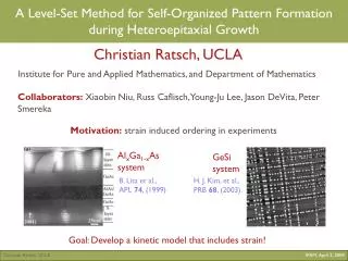
13. Vertical alignment of stacked quantum dots Stacked InAs quantum dots on GaAs(001) • Islands nucleate “on top” of lower islands • Size and separation becomes more uniform • Interpretation: buried islands lead to strain (there is a 7% misfit) • Spatially varying potential energy surface • Spatially varying nucleation probability B. Lita et al. (Goldman group), APL 74, 2824 (1999)

14. Aligned islands due to buried dislocation lines Ge on relaxed SiGe buffer layers • Islands align along lines • Dislocation lines are buried underneath • Interpretation: buried dislocation lines lead to strain • Spatially varying potential energy surface • Spatially varying nucleation probability Level Set formalism is ideally suited to incorporate anisotropic, spatially varying diffusion and thus nucleation without extra computational cost H. J. Kim, Z. M. Zhao, Y. H. Xie, PRB 68, 205312 (2003).

15. Replace diffusion constant by matrix: Diffusion in x-direction Diffusion in y-direction Possible variations of potential energy surface • Diffusion equation: no drift • Velocity: drift • Nucleation Rate: Modifications to the level set formalism for non-constant diffusion

16. fast diffusion slow diffusion Isotropic diffusion with sinusoidal variation in x-direction Only variation of transition energy, and constant adsorption energy • Islands nucleate in regions of fast diffusion • Little subsequent nucleation in regions of slow diffusion

17. Comparison with experimental results Results of Xie et al. (UCLA, Materials Science Dept.) Simulations

18. Isotropic diffusion with sinusoidal variation in x- and y-direction

19. Etran Ead Spatially constant adsorption and transition energies, i.e., no drift small amplitude large amplitude Regions of fast surface diffusion Most nucleation does not occur in region of fast diffusion, but is dominated by drift Anisotropic diffusion with variation of adsorption energy What is the effect of thermodynamic drift ?

20. D x Transition from thermodynamically to kinetically controlled diffusion Constant transition energy (thermodynamic drift) Constant adsorption energy (no drift) In all cases, diffusion constant D has the same form: • No drift (right): nucleation dominated by fast diffusion • Large Drift (left): nucleation dominated by drift

21. Time evolution in the kinetic limit • A properly modified PES (in the “kinetic limit”) leads to very regular, 1-D structures • Can this approach used to produce quantum wires?

22. Combination of island dynamics model with elastic code • In contrast to an atomistic (KMC) simulation, the timestep is rather large, even when we have a large detachment rate (high temperature). • A typical timestep in our simulation is O(10-2 s); compare to typical atomistic simulation, where it is O(10-6 s). • This allows us to do an “expensive calculation” at every timestep. • For example, we can solve the elastic equations at every timestep, and couple the local value of the strain to the microscopic parameters. • This work is currently in progress ….. but here are some initial results.

23. Our Elastic model • Write down an atomistic energy density, that includes the following terms (lattice statics) (this is work by Caflisch, Connell, Luo, Lee, et al.): • Nearest neighbor springs • Diagonal springs • Bond bending terms • This can be related to (and interpreted as) continuum energy density • Minimize energy with respect to all displacements: uE [u]=0

24. Numerical Method • PCG using Algebraic MultiGrid (poster by Young-Ju Lee) • Artificial boundary conditions at top of substrate (poster by Young-Ju Lee) • Additional physics, such as more realistic potential or geometry easily included

25. Sxx Syy Couple elastic code to island dynamics model • Example: • Epilayer is 4% bigger than substrate (I.e., Ge on Si) • Choose elastic constants representative for Ge, Si • Deposit 0.2 monolayers

26. The dependence of D on strain can be based on DFT results. Example: Stain dependent diffusion for Ag/Ag(111) C. Ratsch, A.P. Seitsonen, and M. Scheffler Phys. Rev. B 55, 6750-6753 (1997). Modification of diffusion field

27. Results with strain-dependent detachment rate Constant diffusion Change diffusion as a function of strain at every timestep • It is not clear whether there is an effect on ordering • More quantitative analysis needed

28. Modification of detachment rates • The detachment rate has only physical meaning at the island edge (where it changes the boundary condition req) • The model shown here indicates that it is more likely to detach from a bigger (more strained island) than from a smaller one. • Previous (KMC) work suggests that this leads to more uniform island size distribution.

29. Results with strain-dependent detachment rate No change of Ddet Strain induced change of Ddet at every timestep • Maybe fewer islands are close together upon strain induced increase of Ddet (?) • Obviously, a more quantitative analysis is needed!

30. Conclusions • We have developed a numerically stable and accurate level set method to describe epitaxial growth. • Only the relevant microscopic fluctuations are included. • Fast events can be included without changing the timestep of the simulations. • This framework is ideally suited to include anisotropic, spatially varying diffusion. • A properly modified potential energy surface can be exploited to obtain a high regularity in the arrangement of islands. • We have combined this model with a strain model, to modify the microscopic parameters of the model according to the local value of the strain.

31. Need 4 points to discretize with third order accuracy i+1 i+2 i-1 i i+3 i+4 i-3 i-2 Set 1 Set 2 Set 3 This often leads to oscillations at the interface Fix: pick the best four points out of a larger set of grid points to get rid of oscillations (“essentially-non-oscillatory”) Essentially-Non-Oscillatory (ENO) Schemes

32. Standard Discretization: • Leads to a symmetric system of equations: • Use preconditional conjugate gradient method Problem at boundary: i i-2 i-1 i+1 ; replace by: Matrix not symmetric anymore : Ghost value at i “ghost fluid method” Solution of Diffusion Equation