Download
1 / 15
160 likes | 318 Views
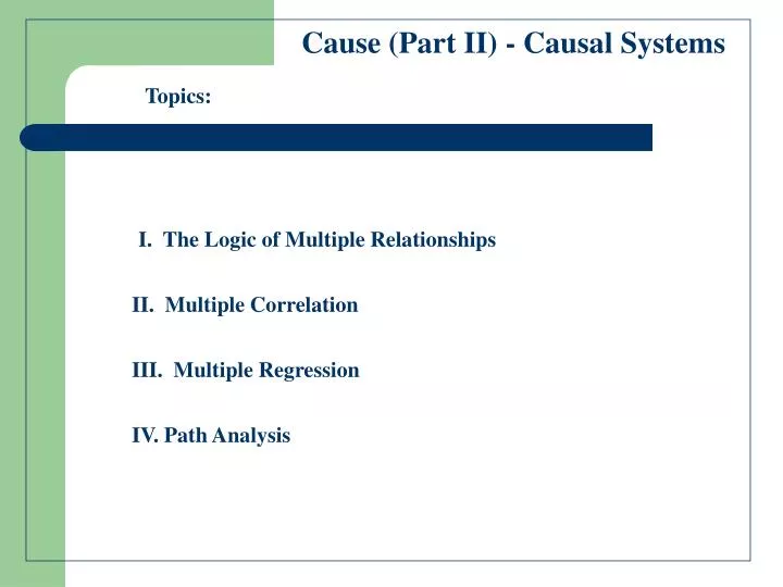
Cause (Part II) - Causal Systems. Topics:. I. The Logic of Multiple Relationships. II. Multiple Correlation. III. Multiple Regression. IV. Path Analysis. Cause (Part II) - Causal Systems. I. The Logic of Multiple Relationships. One Dependent Variable, Multiple Independent Variables.

E N D
Cause (Part II) - Causal Systems Topics: I. The Logic of Multiple Relationships II. Multiple Correlation III. Multiple Regression IV. Path Analysis
Cause (Part II) - Causal Systems I. The Logic of Multiple Relationships One Dependent Variable, Multiple Independent Variables NR X1 Y R NR X2 In this diagram the overlap of any two circles can be thought of as the r2 between the two variables. When we add a third variable, however, we must ‘partial out’ the redundant overlap of the additional independent variables.
Cause (Part II) - Causal Systems II. Multiple Correlation NR X1 Y R X1 NR Y NR X2 NR X2 R2y.x1x2= r2yx1 + r2yx2 R2y.x1x2= r2yx1 + r2yx2.x1 Notice that when the Independent Variables are independent of each other, the multiple correlation coefficient (R2) is simply the sum of the individual r2, but if the independent variables are related, R2 is the sum of one zero order r2 of one plus the partial r2of the other(s). This is required to compensate for the fact that multiple independent variables being related to each other would be otherwise double counted in explaining the same portion of the dependent variable. Partially out this redundancy solves this problem.
Cause (Part II) - Causal Systems II. Multiple Regression Y’ = a + byx1X1 + byx2X2 X1 Y X2 or Standardized X1 Y’ = Byx1X1 + Byx2X2 Y X2 If we were to translate this into the language of regression, multiple independent variables, that are themselves independent of each other would have their own regression slopes and would simply appear as an another term added in the regression equation.
Cause (Part II) - Causal Systems Multiple Regression X1 Y Y’ = a + byx1X1 + byx2.x1X2 or Standardized X2 Y’ = Byx1X1 + Byx2.x1X2 X1 Y X2 Once we assume the Independent Variables are themselves related with respect to the variance explained in the Dependent Variable, then we must distinguish between direct and indirect predictive effects. We do this using partial regression coefficients to find these direct effects. When standardized these B-values are called “Path coefficients” or “Beta Weights”
Cause (Part II) - Causal Systems III. Path Analysis – The Steps and an Example 1. Input the data 2. Calculate the Correlation Matrix 3. Specify the Path Diagram 4. Enumerate the Equations 5. Solve for the Path Coefficients (Betas) 6. Interpret the Findings
Path Analysis – Steps and Example Step1 – Input the data Assume you have information from ten respondents as to their income, education, parent’s education and parent’s income. We would input these ten cases and four variables into SPSS in the usual way, as here on the right. In this analysis we will be trying to explain respondent’s income (Y), using the three other independent variables (X1, X2, X3) Y = DV - income X3 = IV - educ X2 = IV - pedu X1 = IV - pinc
Path Analysis – Steps and Example Step 2 – Calculate the Correlation Matrix These correlations are calculated in the usual manner through the “analyze”, “correlate”, bivariate menu clicks. Notice the zero order correlations of each IV with the DV. Clearly these IV’s must interrelate as the values of the r2 would sum to an R2 indicating more than 100% of the variance in the DV which, of course, is impossible.
Path Analysis – Steps and Example Step 3 – Specify the Path Diagram Therefore, we must specify a model that explains the relationship among the variables across time We start with the dependent variable on the right most side of the diagram and form the independent variable relationship to the left, indicating their effect on subsequent variables. X1 a e Y f X3 b d Y = Offspring’s income c X1 = Parent’s income X2 X2 = Parent’s education X3 = Offspring’s education Time
Path Analysis – Steps and Example Step 4 – Enumerate the Path Equations With the diagram specified, we need to articulate the formulae necessary to find the path coefficients (arbitrarily indicated here by letters on each path). Overall correlations between an independent and the dependent variable can be separated into its direct effect plus the sum of its indirect effects. X1 a e X3 Y f b d 1.ryx1 = a + brx3x1 + crx2x1 c 2.ryx2 = c + brx3x2 + arx1x2 X2 3.ryx3 = b + arx1x3 + crx2x3 4.rx3x2 = d + erx1x2 Click here for solution to two equations in two unknowns 5.rx3x1 = e + drx1x2 6.rx1x2 = f
Path Analysis – Steps and Example Step 5 – Solve for the Path Coefficients The easiest way to calculate B is to use the Regression module in SPSS. By indicating income as the dependent variable and pinc, pedu and educ as the independent variables, we can solve for the Beta Weights or Path Coefficients for each of the Independent Variables. These circled numbers correspond to Beta for paths a, c and b, respectively, in the previous path diagram.
Path Analysis – Steps and Example Step 5a – Solving for R2 The SPSS Regression module also calculate R2. According to this statistic, for our data, 50% of the variation in the respondent’s income (Y) is accounted for by the respondent’s education (X3), parent’s education (X2) and parent’s income (X1) R2 is calculated by multiplying the Path Coefficient (Beta) by its respective zero order correlation and summed across all of the independent variables (see spreadsheet at right).
Path Analysis – Steps and Example Checking the Findings ryx1 = a + brx3x1 + crx2x1 .69 = .63 + -.21(.75) +.31(.68) e = .50 ryx2 = c + brx3x2 + arx1x2 X1 r = .69 B = .63 .57 = .31 + -.21(.82) + .63(.68) r = .75 B = .36 ryx3 = b + arx1x3 + crx2x3 .52 = -.21 + .63(.75) + .31(.82) r = .52 B = -.21 Y X3 r = B =.68 The values of r and B tells us three things: 1) the value of Beta is the direct effect; 2) dividing Beta by r gives the proportion of direct effect; and 3) the product of Beta and r summed across each of the variables with direct arrows into the dependent variable is R2 . The value of 1-R2is e. r = .82 B = .57 r = .57 B =.31 X2 Time
Path Analysis – Steps and Example Step 6 – Interpret the Findings Y = Offspring’s income X3 = Offspring’s education X2 = Parent’s education X1 e = .50 X1 = Parent’s income .63 Specifying the Path Coefficients (Betas), several facts are apparent, among which are that Parent’s income has the highest percentage of direct effect (i.e., .63/.69 = 92% of its correlation is a direct effect, 8% is an indirect effect). Moreover, although the overall correlation of educ with income is positive, the direct effect of offspring’s education, in these data, is actually negative! .36 Y .68 X3 -.21 .57 .31 X2 Time End