Download
1 / 15
190 likes | 943 Views
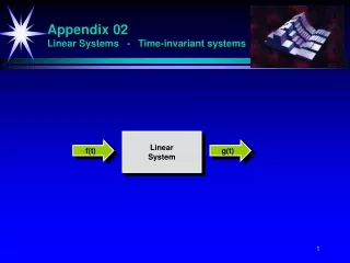
Linear Time-Invariant Systems. Discrete-Time LTI Systems: Convolution Sum Continuous-Time LTI Systems: Convolution Integral Properties of LTI Systems Causal LTI Systems Described by Differential and Difference Equations Singularity Functions. Discrete-Time LTI Systems.

E N D
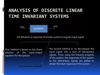
Linear Time-Invariant Systems • Discrete-Time LTI Systems: Convolution Sum • Continuous-Time LTI Systems: Convolution Integral • Properties of LTI Systems • Causal LTI Systems Described by • Differential and Difference Equations • Singularity Functions
Discrete-Time LTI Systems • Representation of Discrete-Time Signals in Terms of Impulses • Discrete-Time Unit Impulse Response and the Convolution-Sum Representation
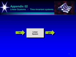
Representation of Discrete-Time Signals in Terms of Impulses Discrete-time unit impulse, , can be used to construct any discrete-time signal Discrete-time signal is a sequence of individual impulses Consider x[n]
5 time shifted impulses scaled by x[n] • Therefore • x[n] = x[-3]δ[n+3] + x[-2]δ[n+2] + x[-1]δ[n+2] + x0]δ[n] + x[1]δ[n-1] + x[2]δ[n-2] + x[3]δ[n-3] • or
Represents arbitrary sequence as linear combination of shifted unit impulses δ[n-k], where the weights are x[k] • Often called the Sifting Property of Discrete-Time unit impulse • Because δ[n-k] is nonzero only when k = n the summation “sifts” through the sequence of values x[k] and preserves only the value corresponding to k = n
Discrete-Time Unit Impulse Response and the Convolution-Sum Representation • Sifting property represents x[n] as a superposition of scaled versions of very simple functions • shifted unit impulses, δ[n-k], each of which is nonzero at a single point in time specified by the corresponding value of k
Response of Linear system will be • Superposition of scaled responses of the system to each shifted impulse • Time Invariance tells us that • Responses of a time-invariant system to • time-shifted unit impulses are • time-shifted versions of one another • Convolution-Sum representation for D-T LTI systems is based on these two facts
Convolution-sum Representation of LTI Systems • Consider response of linear system to x[n] • says input can be represented as linear combination of shifted unit impulses
let hk[n] denote response of linear system to shifted unit impulse δ[n-k] • Superposition property of a linear system says the response y[n] of the linear system to x[n] is weighted linear combination of these responses • with input x[n] to a linear system the output y[n] can be expressed as
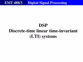
If x[n] is applied to a system Whose responses h-1[n], h0[n], and h1[n] to the signals δ[n+1], δ[n], and δ[n-1] are Superposition allows us to write the response to x[n] as a linear combination of the responses to the individual shifted impulses
x[n] system response to δ[n+1], δ[n], δ[n-1]
Continuous-Time LTI Systems: Convolution Integral • Representation of Continuous-Time Signals in Terms of Impulses • Continous-Time Unit Impulse Response and the Convolution Integral Representation of LTI Systems
Properties of LTI Systems • Commutative Property • Distributive Property • Associative Property • LTI Systems with and without Memory • Invertibility of LTI Systems • Causality of LTI Systems • Stability for LTI Systems • Unit Step Response of an LTI System
Causal LTI Systems Described byDifferential and Difference Equations • Linear Constant-Coefficient Differential Equations • Linear Constant-Coefficient Difference Equations • Block Diagram Representations of First-Order Systems Described by Differential and Difference Equations
Singularity Functions • Unit Impulse as an Idealized Short Pulse • Defining the Unit Impulse through Convolution • Unit Doublets and other Singularity Functions