Download

1 / 24
240 likes | 355 Views
Modelling inflows for water valuation. Dr. Geoffrey Pritchard University of Auckland / EPOC. Inflows – where it all starts. CATCHMENTS. thermal generation. reservoirs. hydro generation. transmission. consumption. We want: inflow scenarios for use with generation/power system models

E N D
Modelling inflows for water valuation Dr. Geoffrey Pritchard University of Auckland / EPOC
Inflows – where it all starts CATCHMENTS thermal generation reservoirs hydro generation transmission consumption We want: inflow scenarios for use with generation/power system models - in a form useful for optimization. Historical inflow sequences work for back-testing of a known strategy - but not for optimization (will be clairvoyant).
Hydro-thermal scheduling • The problem: Operate a combination of hydro and thermal power stations • - meeting demand, etc. • - at least cost (fuel, shortage). • Assume a mechanism (wholesale market, or single system operator) capable of solving this problem.
SDDP for hydro-thermal scheduling Week 7 Week 8 Week 6
SDDP for hydro-thermal scheduling Week 7 Week 8 Week 6 min (present cost) + E[ future cost ] s.t. (satisfy demand, etc.)
SDDP for hydro-thermal scheduling Week 7 Week 8 Week 6 Sps min (present cost) + E[ future cost ] s.t. (satisfy demand, etc.) s The critical step requires estimating expected cost (the “expected future cost” for earlier stages); so uncertainty (from inflows) must be modelled with discrete scenarios. - lognormal, Pearson III, or other continuous distributions won’t do.
Inflow scenarios for a single week (1/7/2014 – 7/7/2014, say) The historical record gives one scenario per historical year - may be too many scenarios, or too few - historical extreme events can recur, but only in the identical week of the year
Scenarios by quantile regression • Each scenario has its own curve. • Any number of scenarios, possibly with unequal probabilities. • - computationally intensive models • Smooth seasonal variation. • - model interpretation
Serial dependence Inflow scenarios for successive weeks should not just be sampled independently.
Serial dependence affects the distribution of total inflow over periods longer than 1 week. (Model simulated for 100 x 62 years, independent weekly inflows.)
Variance inflation • Keep the assumed independence of weekly inflows, but modify their distribution to increase its variance. • Wrong in two ways, but hopefully the errors cancel. • Used e.g. in SPECTRA.
Variance inflation • Keep the assumed independence of weekly inflows, but modify their distribution to increase its variance. • Wrong in two ways, but hopefully the errors cancel. • Used e.g. in SPECTRA.
With variance inflation, inflow distribution is wrong over 1 week – but not bad over 4 months. (Model simulated for 100 x 62 years, independent weekly inflows with vif=2.2.)
Explicit serial dependence • Inflow is a random linear (or concave) function of inflow (or a state variable) from previous stage(s): • Xt = Ft(Xt-1) (Ft random, i.e. scenario-dependent) • Commonest type is log-autoregressive: • log Xt = b log Xt-1 + a + et (et random) • General linear form (ideal for SDDP): • Xt = At + BtXt-1 (At, Bt random)
Serially dependent models 62 scenarios derived from regression residuals 16 scenarios fitted by quantile regression Models fitted to all data, shown for week beginning 2013-08-31
Serially dependent model can match inflow distribution over 1-week and 4-month timescales. (Model simulated for 100 x 62 years, dependent weekly inflows, general linear form.)
A test problem • Challenging fictional system based on Waitaki catchment inflows. • Storage capacity 1000 GWh (cf. real Waitaki lakes 2800 GWh) • Generation capacity 1749 MW hydro, 900 MW thermal • Demand 1550 MW, constant • Thermal fuel $50 / MWh, VOLL $1000 / MWh • Test problem: a dry winter. • 35 weeks (2 April – 2 December) • Initial storage 336 GWh • Initial inflow 500 MW (~56% of average) • Solved with Doasa 2.0 (EPOC’s SDDP code).
Results – optimal strategy (Quantities are expected averages over full time horizon; probabilities are for any shortage/spill within time horizon.)