Download
1 / 24
240 likes | 464 Views
A Simple Inventory System. Modeling and Simulation CS 313. A simple inventory system. Conceptual Model Transaction Reporting Inventory review after each transaction Significant labor may be required Less likely to experience shortage Periodic Inventory Review

E N D
A Simple Inventory System Modeling and Simulation CS 313
A simple inventory system • Conceptual Model • Transaction Reporting • Inventory review after each transaction • Significant labor may be required • Less likely to experience shortage • Periodic Inventory Review • Inventory review is periodic • Items are ordered, if necessary, only at review times • (s, S) are the min, max inventory levels, 0 ≤ s < S • We assume periodic inventory review • Search for (s, S) that minimize cost
A simple inventory system • Conceptual Model • Inventory System Costs • Holding cost: for items in inventory • Shortage cost: for unmet demand • Setup cost: fixed cost when order is placed • Item cost: per-item order cost • Ordering cost: sum of setup and item costs • Additional Assumptions • Back ordering is possible • No delivery lag • Initial inventory level is S • Terminal inventory level is S
A simple inventory system Specification Model Time begins at t = 0 Review times are t = 0, 1, 2, . . . li−1 : inventory level at beginning of ithinterval oi−1 : amount ordered at time t = i − 1, (oi−1 ≥ 0) di : demand quantity during ith interval, (di ≥ 0) Inventory at end of interval can be negative
A simple inventory system • Inventory Level Considerations: • Inventory level is reviewed at t = i − 1 • If at least s, no order is placed • If less than s, inventory is replenished to S • Items are delivered immediately • At end of ithinterval, inventory diminished by di • li = li−1 + oi−1 − di
Example 1.3.1: SIS with sample demands Let (s, S) = (20, 60) and consider n = 12 time intervals
Output statistics • What statistics to compute? • Average demand and average order • For Example 1.3.1 data • = = 305/12 ≃ 25.42 items per time interval.
Flow Balance Average demand and order must be equal Ending inventory level is S Over the simulated period, all demand is satisfied Average “flow” of items in equals average “flow” of items out The inventory system is flow balanced
Constant Demand Rate Holding and shortage costs are proportional to time-averaged inventory levels Must know inventory level for all t Assume the demand rate is constant between review times
Inventory level as a function of time The inventory level at any time t in ith interval is l(t) = l′i−1 − (t − i + 1) di If demand rate is constant between review times l′i−1 = li−1 + oi−1 represents inventory level after review
Inventory decrease is not linear Inventory level at any time t is an integer l(t) should be rounded to an integer value l(t) is a stair-step, rather than linear, function
Time-Averaged Inventory Level l(t) is the basis for computing the time-averaged inventory level Case 1: if l(t) remains non-negative over ithinterval Case 2: if l(t) becomes negative at some time  ̄l+iis the time-averaged holding level  ̄l−iis the time-averaged shortage level
TIME-AVERAGED INVENTORY LEVEL Time-averaged holding level and time-averaged shortage level The time-averaged inventory level is
COMPUTATIONAL MODEL sis1 is a trace-driven computational model of the SIS Computes the statistics  ̄d,  ̄o,  ̄l +,  ̄l − and the order frequency  ̄u Consistency check: compute  ̄o and  ̄d separately, then compare
EXAMPLE 1.3.4: EXECUTING SIS1 Trace file sis1.dat contains data for n = 100 time intervals With (s, S) = (20, 80)
OPERATING COSTS A facility’s cost of operation is determined by:
CASE STUDY Full Example at Page 33 in the book… Automobile dealership that uses weekly periodic inventory review The facility is the showroom and surrounding areas The items are new cars The supplier is the car manufacturer “...customers are people convinced by clever advertising that their lives will be improved significantly if they purchase a new car from this dealer.” (S. Park) Simple (one type of car) inventory system
EXAMPLE 1.3.5: CASE STUDY MATERIALIZED Limited to a maximum of S = 80 cars Inventory reviewed every Monday If inventory falls below s = 20, order cars sufficient to restore to S For now, ignore delivery lag Costs:
PER-INTERVAL AVERAGE OPERATING COSTS The average operating costs per time interval are The average total operating cost per time interval is their sum For the stats and costs of the hypothetical dealership:
COST MINIMIZATION • By varying s (and possibly S), an optimal policy can be determined • Optimal ⇐⇒ minimum average cost • Note that  ̄o =  ̄d, and  ̄d depend only on the demands • Hence, item cost is independent of (s, S) • Average dependent cost is avg setup cost + avg holding cost + avg shortage cost • Let S be fixed, and let the demand sequence be fixed • If s is systematically increased, we expect: • Average setup cost and holding cost will increase as s increases • Average shortage cost will decrease as s increases • Average dependent cost will have ‘U’ shape, yielding an optimum