Loop Unrolling

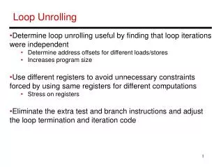
1. Loop Unrolling • Determine loop unrolling useful by finding that loop iterations were independent • Determine address offsets for different loads/stores • Increases program size • Use different registers to avoid unnecessary constraints forced by using same registers for different computations • Stress on registers • Eliminate the extra test and branch instructions and adjust the loop termination and iteration code

2. Loop Unrolling • If a loop only has dependences within an iteration, the loop • is considered parallel  multiple iterations can be executed • together so long as order within an iteration is preserved • If a loop has dependences across iterations, it is not parallel • and these dependences are referred to as “loop-carried”

3. Example For (i=1000; i>0; i=i-1) x[i] = x[i] + s; For (i=1; i<=100; i=i+1) { A[i+1] = A[i] + C[i]; S1 B[i+1] = B[i] + A[i+1]; S2 } For (i=1; i<=100; i=i+1) { A[i] = A[i] + B[i]; S1 B[i+1] = C[i] + D[i]; S2 } For (i=1000; i>0; i=i-1) x[i] = x[i-3] + s; S1

4. Example For (i=1000; i>0; i=i-1) x[i] = x[i] + s; No dependences For (i=1; i<=100; i=i+1) { A[i+1] = A[i] + C[i]; S1 B[i+1] = B[i] + A[i+1]; S2 } S2 depends on S1 in the same iteration S1 depends on S1 from prev iteration S2 depends on S2 from prev iteration For (i=1; i<=100; i=i+1) { A[i] = A[i] + B[i]; S1 B[i+1] = C[i] + D[i]; S2 } S1 depends on S2 from prev iteration S1 depends on S1 from 3 prev iterations Referred to as a recursion Dependence distance 3; limited parallelism For (i=1000; i>0; i=i-1) x[i] = x[i-3] + s; S1

5. Constructing Parallel Loops If loop-carried dependences are not cyclic (S1 depending on S1 is cyclic), loops can be restructured to be parallel For (i=1; i<=100; i=i+1) { A[i] = A[i] + B[i]; S1 B[i+1] = C[i] + D[i]; S2 } A[1] = A[1] + B[1]; For (i=1; i<=99; i=i+1) { B[i+1] = C[i] + D[i]; S3 A[i+1] = A[i+1] + B[i+1]; S4 } B[101] = C[100] + D[100]; S1 depends on S2 from prev iteration S4 depends on S3 of same iteration Loop unrolling reduces impact of branches on pipeline; another way is branch prediction

6. Static Branch Prediction • Scheduling code around delayed branch • To reorder code around branches, need to predict branch statically at compile time • Simplest scheme is to predict a branch as taken • Average misprediction = untaken branch frequency = 34% SPEC • More accurate scheme predicts branches using profile information collected from earlier runs, and modify prediction based on last run:

7. Dynamic Branch Prediction • Why does prediction work? • Underlying algorithm has regularities • Data that is being operated on has regularities • Is dynamic branch prediction better than static branch prediction? • Seems to be • There are a small number of important branches in programs which have dynamic behavior

8. Dynamic Branch Prediction • Performance = ƒ(accuracy, cost of misprediction) • Branch History Table: Lower bits of PC address index table of 1-bit values • Says whether or not branch taken last time • No address check • Problem: in a loop, 1-bit BHT will cause two mispredictions • End of loop case, when it exits instead of looping as before • First time through loop on next time through code, when it predicts exit instead of looping

9. Dynamic Branch Prediction • Solution: 2-bit scheme where change prediction only if get misprediction twice • More sophisticated • Count the number of times branch is taken 2-bit branch prediction State diagram

10. Branch History Table • Mispredict because either: • Wrong guess for that branch • Got branch history of wrong branch when index the table • 4096 entry table:

11. Correlated Branch Prediction • Standard 2-bit predictor uses local information • Fails to look at the global picture • Idea: record m most recently executed branches as taken or not taken, and use that pattern to select the proper n-bit branch history table • Global Branch History: m-bit shift register keeping T/NT status of last m branches.

12. Correlated Branch Prediction • Hypothesis: recent branches are correlated; that is, behavior of recently executed branches affects prediction of current branch • Idea: record m most recently executed branches as taken or not taken, and use that pattern to select the proper branch history table • In general, (m,n) predictor means record last m branches to select between 2^m history tables each with n-bit counters • Old 2-bit BHT is then a (0,2) predictor • If (aa == 2) • aa=0; • If (bb == 2) • bb = 0; • If (aa != bb) • do something;

13. Correlated Branch Prediction • (2,2) predictor • Then behavior of recent branches selects between, say, four predictions of next branch, updating just that prediction

14. Accuracy of Different Schemes 20% 4096 Entries 2-bit BHT Unlimited Entries 2-bit BHT 1024 Entries (2,2) BHT 18% 16% 14% 12% 11% Frequency of Mispredictions 10% 8% 6% 6% 6% 6% 5% 5% 4% 4% 2% 1% 1% 0% 0% nasa7 matrix300 tomcatv doducd spice fpppp gcc expresso eqntott li 4,096 entries: 2-bits per entry Unlimited entries: 2-bits/entry 1,024 entries (2,2)

15. Tournament Predictors • Multilevel branch predictor • Selector for the Global and Local predictors of correlating branch prediction • Use n-bit saturating counter to choose between predictors • Usual choice between global and local predictors

16. Tournament Predictors • A local predictor might work well for some branches or • programs, while a global predictor might work well for others • Provide one of each and maintain another predictor to • identify which predictor is best for each branch Local Predictor M U X Global Predictor Branch PC Tournament Predictor Table of 2-bit saturating counters

17. Tournament Predictors • Tournament predictor using, say, 4K 2-bit counters indexed by local branch address. Chooses between: • Global predictor • 4K entries index by history of last 12 branches (2^12 = 4K) • Each entry is a standard 2-bit predictor • Local predictor • Local history table: 1024 10-bit entries recording last 10 branches, index by branch address • The pattern of the last 10 occurrences of that particular branch used to index table of 1K entries with 3-bit saturating counters

18. Tournament Predictors • Advantage of tournament predictor is ability to select the right predictor for a particular branch

19. 1-Bit Bimodal Prediction (SimpleScalar Term) • For each branch, keep track of what happened last time • and use that outcome as the prediction • What are prediction accuracies for branches 1 and 2 below: • while (1) { • for (i=0;i<10;i++) { branch-1 • … • } • for (j=0;j<20;j++) { branch-2 • … • } • }

20. 2-Bit Bimodal Prediction (SimpleScalar Term) • For each branch, maintain a 2-bit saturating counter: • if the branch is taken: counter = min(3,counter+1) • if the branch is not taken: counter = max(0,counter-1) • If (counter >= 2), predict taken, else predict not taken • Advantage: a few atypical branches will not influence the • prediction (a better measure of “the common case”) • Especially useful when multiple branches share the same • counter (some bits of the branch PC are used to index • into the branch predictor) • Can be easily extended to N-bits (in most processors, N=2)

21. Branch Target Buffers (BTB) • Branch target calculation is costly and stalls the instruction fetch. • BTB stores PCs the same way as caches • The PC of a branch is sent to the BTB • When a match is found the corresponding Predicted PC is returned • If the branch was predicted taken, instruction fetch continues at the returned predicted PC

22. Branch Target Buffers (BTB)

23. Branch Prediction • Sophisticated Techniques: • A “branch target buffer” to help us look up the destination • Correlating predictors that base prediction on global behaviorand recently executed branches (e.g., prediction for a specificbranch instruction based on what happened in previous branches) • Tournament predictors that use different types of prediction strategies and keep track of which one is performing best. • A “branch delay slot” which the compiler tries to fill with a useful instruction (make the one cycle delay part of the ISA) • Branch prediction is especially important because it enables other more advanced pipelining techniques to be effective! • Modern processors predict correctly 95% of the time!

24. Pipeline without Branch Predictor PC IF (br) Reg Read Compare Br-target PC + 4 In the 5-stage pipeline, a branch completes in two cycles  If the branch went the wrong way, one incorrect instr is fetched  One stall cycle per incorrect branch

25. Pipeline with Branch Predictor PC IF (br) Reg Read Compare Br-target Branch Predictor In the 5-stage pipeline, a branch completes in two cycles  If the branch went the wrong way, one incorrect instr is fetched  One stall cycle per incorrect branch

26. Branch Mispredict Penalty • Assume: no data or structural hazards; only control • hazards; every 5th instruction is a branch; branch • predictor accuracy is 90% • Slowdown = 1 / (1 + stalls per instruction) • Stalls per instruction = % branches x %mispreds x penalty • = 20% x 10% x 1 • = 0.02 • Slowdown = 1/1.02 ; if penalty = 20, slowdown = 1/1.4

27. Dynamic Vs. Static ILP • Static ILP: • + The compiler finds parallelism  no extra hw  higher clock speeds and lower power + Compiler knows what is next  better global schedule - Compiler can not react to dynamic events (cache misses) - Can not re-order instructions unless you provide hardware and extra instructions to detect violations (eats into the low complexity/power argument) - Static branch prediction is poor  even statically scheduled processors use hardware branch predictors

28. Dynamic Scheduling • Hardware rearranges instruction execution to reduce stalls • Maintains data flow and exception behavior • Advantages: • Handles cases where dependences are unknown at compile time • Simplifies compiler • Allows processor to tolerate unpredictable delays by executing other code • Cache miss delay • Allows code compiled with one pipeline in mind to run efficiently on a different pipeline • Disadvantage: • Complex hardware

29. Dynamic Scheduling • Simple Pipelining technique: • In-order instruction issue and execution • If an instruction is stalled, no later instructions can proceed • Dependence between two closely spaced instructions leads to hazard • What if there are multiple functional units? • Units could stay idle • If instruction “j” depends on a long running instruction “i” • All instructions after “j” stalls Can be eliminated by not requiring instructions to execute in-order DIV.D F0,F2,F4 ADD.D F10,F0,F8 SUB.D F12,F8,F14

30. Idea • Classic five stage pipeline • Structural and data hazards could be checked during ID • What do we need to allow us execute the SUB.D? • Separate ID process into two • Check for hazards (Issue) • Decode (read operands) • In-order instruction issue (in program order) • Begin execution as soon as its operands are available • Out-of-order execution (out-of-order completion) DIV.D F0,F2,F4 ADD.D F10,F0,F8 SUB.D F12,F8,F14

31. Out-of-order complications • Introduces possibility of WAW, WAR hazards • Do not exist in 5 stage pipeline • Solution • Register renaming DIV.D F0,F2,F4 ADD.D F6,F0,F8 SUB.D F8,F10,F14 MUL.D F6,F10,F8 WAR WAW

32. Out-of-order complications • Handling exceptions • Out-of-order completion must preserve exception behavior • Exactly those exceptions that would arise if the program was executed in strict program order actually do arise • Preserve exception behavior by: • Ensuring that no instruction can generate an exception until the processor knows that the instruction raising the exception will be executed

33. Splitting ID Stage • Instruction Fetch: • Fetch into register or queue • Instruction Decode • Issue: • Decode instructions • Check for structural hazards • Read operands • Wait until no data hazards • Then read operands • Execute • Just as 5-stage pipeline execute stage • May take multiple cycles

34. Hardware requirement • Pipeline must allow multiple instructions to be in execution stage • Multiple functional units • Instructions pass through issue stage in order (in-order issue) • Instructions can be stalled and bypass each other in the second stage (read operands) • Instructions enter execution stage out-of-order

35. Dynamic Scheduling using Tomasulo’s Method • Sophisticated scheme to allow out-of-order execution • Objective is to minimize RAW hazards • Introduces register renaming to minimize WAR and WAW hazards • Many variations of this technique are used in modern processors • Common features: • Tracking instruction dependencies to allow as soon as (only when) operands are available (resolves RAW) • Renaming destination registers (WAR, WAW)

36. Dynamic Scheduling using Tomasulo’s Method • Register renaming: DIV.D F0,F2,F4 ADD.D F6,F0,F8 S.D F6,0(R1) SUB.D F8,F10,F14 MUL.D F6,F10,F8 DIV.D F0,F2,F4 ADD.D S,F0,F8 S.D S,0(R1) SUB.D T,F10,F14 MUL.D F6,F10,T Finding any use of F8 requires sophisticated compiler or hardware

37. Dynamic Scheduling using Tomasulo’s Method • Register renaming is provided by reservation stations • Buffer the operands of instructions waiting to issue • Reservation station fetches and buffers an operand as soon as it is available • Eliminates the need to get the operand from a register • Pending instructions designate the reservation station that will provide their input (register renaming) • Successive writes to a register: last one is used to update • There can be more reservations stations than real registers! • Name dependencies that can’t be eliminated by a compiler , now can be eliminated by hardware

38. Dynamic Scheduling using Tomasulo’s Method • Data structures attached to • reservation stations • Load/store buffers • Register file • Once an instruction has issued and is waiting for source operand • Refers to the operand by reservation station number where the instruction that will generate the value has been assigned • If reservation statin number is 0 • Operand is already in the register file • 1 cycle latency between source and result • Effective latency between producing instruction and consuming instruction is at least 1 cycle longer than the latency of the function unit producing the result

39. Reservation Station • Op: Operation to perform in the unit (e.g., + or –) • Vj, Vk: Value of Source operands • For loads Vk is used to hold the offset • Qj, Qk: Reservation stations producing source registers (value to be written) • Note: Qj,Qk=0 => ready • Busy: Indicates reservation station or FU is busy • A : Hold information for the memory address calculation for load/store. • Initially, immediate value is stored in A. • Register result status (Qi)—Indicates the number of the reservation station that contains the operation whose results shoul dbe streod in to this register. • Blank when no pending instructions that will write that register.

40. Dynamic Scheduling using Tomasulo’s Method

41. D. Patterson’s Tomasulo Slides

42. Hardware-Based Speculation • Branch prediction reduces the stalls attributable to branches • For a processor executing multiple instructions • Just predicting branch is not enough • Multiple issue processor may execute a branch every clock cycle • Exploiting parallelism requires that we overcome the limitation of control dependence

43. Hardware-Based Speculation • Greater ILP: Overcome control dependence by hardware speculating on outcome of branches and executing program as if guesses were correct • extension over branch prediction with dynamic scheduling • Speculation fetch, issue, and execute instructions as if branch predictions were always correct • Dynamic scheduling only fetches and issues instructions • Essentially a data flow execution model: Operations execute as soon as their operands are available

44. Hardware-Based Speculation • 3 components of HW-based speculation: • Dynamic branch prediction to choose which instructions to execute • Speculation to allow execution of instructions before control dependences are resolved • ability to undo effects of incorrectly speculated sequence • Dynamic scheduling to deal with scheduling of different combinations of basic blocks • without speculation only partially overlaps basic blocks • requires that a branch be resolved before actually executing any instructions in the successor basic block.

45. Hardware-Based Speculation in Tomasulo • The key idea • allow instructions to execute out of order • force instructions to commit in order • prevent any irrevocable action (such as updating state or taking an exception) until an instruction commits. • Hence: • Must separate execution from allowing instruction to finish or “commit” • instructions may finish execution considerably before they are ready to commit. • This additional step called instruction commit

46. Hardware-Based Speculation in Tomasulo • When an instruction is no longer speculative, allow it to update the register file or memory • Requires additional set of buffers to hold results of instructions that have finished execution but have not committed : reorder buffer (ROB) • This reorder buffer (ROB) is also used to pass results among instructions that may be speculated

47. Reorder Buffer • In Tomasulo’s algorithm, once an instruction writes its result, any subsequently issued instructions will find result in the register file • With speculation, the register file is not updated until the instruction commits • (we know definitively that the instruction should execute) • Thus, the ROB supplies operands in interval between completion of instruction execution and instruction commit • ROB is a source of operands for instructions, just as reservation stations (RS) provide operands in Tomasulo’s algorithm • ROB extends architectured registers like RS

48. Reorder Buffer Structure (Four fields) • instruction type field • Indicates whether the instruction is a branch (and has no destination result), a store (which has a memory address destination), or a register operation (ALU operation or load, which has register destinations). • destination field • supplies the register number (for loads and ALU operations) or the memory address (for stores) where the instruction result should be written. • value field • hold the value of the instruction result until the instruction commits. • ready field • indicates that the instruction has completed execution, and the value is ready.

49. Reorder Buffer FP Op Queue FP Regs Res Stations Res Stations FP Adder FP Adder Reorder Buffer Operation • Holds instructions in FIFO order, exactly as issued • When instructions complete, results placed into ROB • Supplies operands to other instruction between execution complete & commit => more registers like RS • Tag results with ROB buffer number instead of reservation station • Instructions commit =>values at head of ROB placed in registers • As a result, easy to undo speculated instructions on mispredicted branches or on exceptions Commit path