Download
1 / 18
250 likes | 542 Views
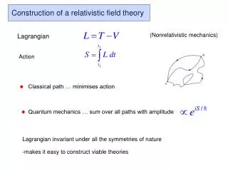
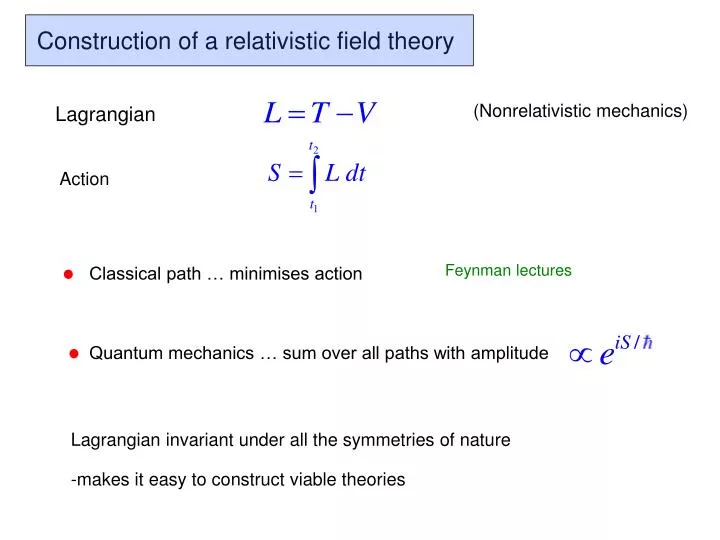
Construction of a relativistic field theory. (Nonrelativistic mechanics). Lagrangian. Action. Feynman lectures. Classical path … minimises action. Quantum mechanics … sum over all paths with amplitude. Lagrangian invariant under all the symmetries of nature.

E N D
Construction of a relativistic field theory (Nonrelativistic mechanics) Lagrangian Action Feynman lectures Classical path … minimises action Quantum mechanics … sum over all paths with amplitude Lagrangian invariant under all the symmetries of nature -makes it easy to construct viable theories
Lagrangian formulation of the Klein Gordon equation Klein Gordon field Manifestly Lorentz invariant } } T V Classical path : Dimensions? Euler Lagrange equation
Euler Lagrange equs Principle of least action : 0 (surface integral) Euler Lagrange equation
Lagrangian formulation of the Klein Gordon equation Klein Gordon field Manifestly Lorentz invariant } } T V Euler Lagrange equation Klein Gordon equation
The Lagrangian and Feynman rules Associate with the various terms in the Lagrangian a set of propagators and vertex factors The propagators determined by terms quadratic in the fields, using the Euler Lagrange equations. The remaining terms in the Lagrangian are associated with interaction vertices. The Feynman vertex factor is just given by the coefficient of the corresponding term in }
Fundamental experimental objects (Dimension 1/T=M) Decay width = 1/lifetime (Dimension L2=M-2) Cross section Units “barn” (Natural Units
Fundamental experimental objects (Dimension 1/T=M) Decay width = 1/lifetime (Dimension L2=M-2) Cross section Transition rate x Number of final states Cross section = Initial flux
Fundamental experimental objects (Dimension 1/T=M) Decay width = 1/lifetime (Dimension L2=M-2) Cross section Momenta of final state forms phase space Transition rate x Number of final states Cross section = Initial flux For a single particle the number of final states in volume V with momenta in element is
Fundamental experimental objects Decay width = 1/lifetime Cross section Transition rate x Number of final states Cross section = Initial flux # target particles per unit volume # particles passing through unit area in unit time (Lab frame)
C A B D The transition rate e.g. Transition rate per unit volume
The cross section Transition rate x Number of final states Cross section = Initial flux Lorentz Invariant Phase space
External photon Compton scattering of a π meson Klein Gordon Feynman rules