Download
1 / 26
260 likes | 338 Views
H ighl Y Constrained Back PR ojection ( HYPR ). Thank you to Oliver Wieben!!. H ighl Y Constrained Back PR ojection ( HYPR ). 1. 3. 5. 7. 9. ‘Composite’. K-space. time. H ighl Y Constrained Back PR ojection ( HYPR ). An approximate acquisition and reconstruction method

E N D
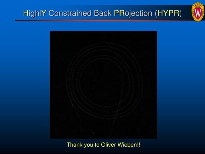
HighlY Constrained Back PRojection (HYPR) Thank you to Oliver Wieben!!
HighlY Constrained Back PRojection (HYPR) 1 3 5 7 9 ‘Composite’ K-space time
HighlY Constrained Back PRojection (HYPR) • An approximate acquisition and reconstruction method • Images should be sparse (few pixels w/signal) • No movement allowed! • Fairly high spatio-temporal correlations • Radial under-sampling at each time frame • Decrease total scan time • Improve temporal resolution • Composite image • Combines data from many time frames • Allows higher SNR for each time frame • Constrains the backprojection reconstruction for each time frame which reduces streak artifacts Mistretta, et al., MRM 55:30-40;2006
Interleaving – Dynamic Imaging 1. Acquire data in interleaves Highly undersample each time frame signal vein artery 1 2 3 4 5 6 7 8 9 …. K-space CE-MRA time
All Inclusive Composite 2. Calculate composite images Sum of ALL projections through time 1 2 3 4 5 6 7 8 9 …. K-space All inclusive composite
Sliding Composite 2. Calculate composite images Sum of “some” projections through time 1 2 3 4 5 6 7 8 9 …. K-space
Sliding Composite 2. Calculate composite images Sum of “some” projections through time 1 2 3 4 5 6 7 8 9 …. K-space
Sliding Composite 2. Calculate composite images Sum of “some” projections through time 1 2 3 4 5 6 7 8 9 …. K-space
All-inclusive versus Sliding Composite Sliding Composite • Lower SNR • More streak artifacts + Better separates early and late filling vessels All-inclusive Composite + High SNR + Few streak artifacts Good for nearly homogeneous temporal behaviour • In CE-MRA: contains early and late filling vessels The SNR of the composite dictates the SNR in the time-resolved images
Time frames with interleaved angular projections time k-space projections 2 N 1 1D FT 1D FT 1D FT 1D FT Image-space projections 2 N 1 Filtered backproject. or sum, regrid, and FT Unfiltered backproject. Composite image . p å = H C p Radon + Unfiltered backprojection c i HYPR time frame N P Pc P/Pc Sum over all projections Multiply
Time frames with interleaved angular projections time k-space projections 2 N 1 1D FT 1D FT 1D FT 1D FT Image-space projections 2 N 1 Filtered backproject. or sum, regrid, and FT Unfiltered backproject. . p Composite image å = H C p Radon + Unfiltered backprojection c i HYPR time frame N P Pc P/Pc Sum over all projections Multiply
Two Vessels – Horizontal – All-inclusive Input (Truth) Schematic × = Composite Weighting HYPR F. Korosec & Y. Wu
Two Vessels – Vertical – All-inclusive Input (Truth) Schematic Wrong! × = Composite Weighting HYPR F. Korosec & Y. Wu
More Projections per HYPR Time Frame 4 Projections 1 Projection Weighting HYPR Weighting HYPR 2 Projections 8 Projections Weighting HYPR Weighting HYPR F. Korosec & Y. Wu
Input Curves and Vessel Locations Input Curves Vessel Locations F. Korosec & Y. Wu
Composite Image #5 Composite 100 projections 5 frames x 20proj/frame Input Curves Time frame #5 Time Frame #5 F. Korosec & Y. Wu
Composite Image #5 Composite 100 projections 5 frames x 20proj/frame Input Curves Time frame #11 Time Frame #11 F. Korosec & Y. Wu
Time Curves – Input and HYPR Input HYPR F. Korosec & Y. Wu
HYPR Simulation Parameters • Gd-doped water injected in tube • 2D Fourier acquisition @ 1 frame / s • Generate k-space projections from images (Matlab) • Simulate HYPR acquisition • 32 projections per interleave • 8 unique sets of interleaves • -> 256 angles sampled • Composite image: moving window [-4 .. +3]
Simulation – Time Frame 5 Original Undersampled Composite HYPR
Simulation – Time Frame 9 Original Undersampled Composite HYPR
Comparison Videos: Foot Undersampled 16 projections per time frame DT = 2.0 s HYPR DT = 2.0 s
Comparison Videos: Calfs Undersampled 16 projections per time frame DT = 2.1 s HYPR DT = 2.1 s • FOV = 48 cm, BW = 62.5 kHz, flip = 25 deg. • TR/TE = 5.2 / 1.1 ms • HYPR frame rate = 2.1 s • Composite: sliding window (duration: 16*2 = 32s)
Applications HYPR Applications • Dynamic Contrast-enhanced MR Angiography • Quantitative Flow Imaging • Diffusion Tensor Imaging • MR and CT Perfusion Imaging • Cardiac Function
HYPR Summary • Improves temporal resolution (also reduces total imaging time) • Improves SNR by incorporation of a time averaged composite image • Small number of projections are used to produce weighting images that are multiplied by high SNR composite image • Composite image constrains backprojection to reduce streak artifacts • Degree of achievable undersampling depends on • sparsity • spatio-temporal correlation • acceptable error