Download
1 / 16
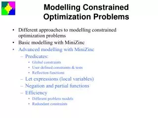
430 likes | 1.34k Views
Optimality conditions for constrained local optima, Lagrange multipliers and their use for sensitivity of optimal solutions . Constrained optimization. Inequality constraints. g2(x ). x 2. g1(x). Infeasible regions. Optimum. Decreasing f(x). x 1. Feasible region. Equality constraints.

E N D
Optimality conditions for constrained local optima, Lagrange multipliers and their use for sensitivity of optimal solutions
Constrained optimization • Inequality constraints g2(x) x2 g1(x) Infeasible regions Optimum Decreasing f(x) x1 Feasible region
Equality constraints • We will develop the optimality conditions for equality constraints and then generalize them for inequality constraints • Give an example of an engineering equality constraint.
Lagrangian and stationarity • Lagrangian function where j are unknown Lagrange multipliers • Stationary point conditions for equality constraints:
Example • Quadratic objective and constraint • Lagrangian • Stationarity conditions • Four stationary points
Problem Lagrange multipliers • Solve the problem of minimizing the surface area of a cylinder of given value V. The two design variables are the radius and height. The equality constraint is the volume constraint.
Inequality constraints • Inequality constraints require transformation to equality constraints: • This yields the following Lagrangian: • Why is the slack variable squared?
Karush-Kuhn-Tucker conditions • Conditions for stationary points are then: • If inequality constraint is inactive (t ≠ 0) then Lagrange multiplier = 0 • For minimum, non-negative multipliers
Convex problems • Convex optimization problem has • convex objective function • convex feasible domain if the line segment connecting any two feasible points is entirely feasible. • All inequality constraints are convex (or gj= convex) • All equality constraints are linear • only one optimum • Karush-Kuhn-Tucker conditions necessary and will also be sufficient for global minimum • Why do the equality constraints have to be linear?
Example extended to inequality constraints • Minimize quadratic objective in a ring • Is feasible domain convex? • Example solved with fmincon using two functions: quad2 for the objective and ring for constraints (see note page)
Message and solution Warning: The default trust-region-reflective algorithm does not solve …. FMINCON will use the active-set algorithm instead. Local minimum found …. Optimization completed because the objective function is non-decreasing in feasible directions, to within the default value of the function tolerance, and constraints are satisfied to within the default value of the constraint tolerance. x =10.0000 -0.0000 fval =100.0000 lambda = lower: [2x1 double] upper: [2x1 double] eqlin: [0x1 double] eqnonlin: [0x1 double] ineqlin: [0x1 double] ineqnonlin: [2x1 double] lambda.ineqnonlin’=1.0000 0 What assumption Matlab likely makes in selecting the default value of the constraint tolerance?
Problem inequality • Solve the problem of minimizing the surface area of the cylinder subject to a minimum value constraint as an inequality constraint. Do also with Matlab by defining non-dimensional radius and height using the cubic root of the volume.
Sensitivity of optimum solution to problem parameters • Assuming problem objective and constraints • depend on parameter p • The optimum solution is x*(p) • The corresponding function value f*(p)=f(x*(p),p)
Sensitivity of optimum solution to problem parameters (contd.) We would like to obtain derivatives of f* w.r.t. p After manipulating governing equations we obtain Lagrange multipliers called “shadow prices” because they provide the price of imposing constraints Why do we have ordinary derivative on the left side and partial on the right side?
Example • A simpler version of ring problem • For p=100 we found • Here it is easy to see that solution is • Which agrees with
Problems sensitivity of optima • For find the optimum for p=0, estimate the derivative df*/dp there, and check by solving again for p=0.1 and comparing to finite difference derivative • Check in a similar way the derivative of the surface area with respect to 1% change in volume (once from the Lagrange multiplier, and once from finite difference of exact solution).