Download
1 / 30
300 likes | 308 Views
Explore the spectral performance metrics for analyzing frequency domain non-ideality in converters or building blocks. Understand the static and dynamic errors and their contribution to non-idealities. Learn about SNR, SNDR, ENOB, DR, SFDR, THD, ERBW, IMD, and MTPR.

E N D
Dynamic Specifications • Spectral performance metrics follow from looking at converter or building block output spectrum • Basic idea: • Apply one or more tones at converter input • Expect same tone(s) at output, all other frequency components represent non-idealities • Important to realize that both static and dynamic errors contribute to frequency domain non-ideality • Static: DNL,INL • Dynamic: glitch impulse, aperture uncertainty, settling time, …
Spectral Metrics • SNR - Signal-to-noise ratio • SNDR (SINAD) - Signal-to-(noise + distortion) ratio • ENOB - Effective number of bits • DR - Dynamic range • SFDR - Spurious free dynamic range • THD - Total harmonic distortion • ERBW - Effective Resolution Bandwidth • IMD - Intermodulation distortion • MTPR - Multi-tone power ratio
Discrete Fourier Transform Basics • DFT takes a block of N time domain samples (spaced Ts=1/fs) and yields a set of N frequency bins • Bin k represents frequency content at k·fs/N [Hz] • DFT frequency resolution • Proportional to 1/(N·Ts) in [Hz/bin] • N·Ts is total time spent gathering samples • A DFT with N=2integer can be found using a computationally efficient algorithm • FFT = Fast Fourier Transform
MATLAB Example clear; N = 100; fs = 1000; fx = 100; x = cos(2*pi*fx/fs*[0:N-1]); s = abs(fft(x)); plot(s 'linewidth' 2);
Normalized Plot with Frequency Axis N = 100; fs = 1000; fx = 100; % full-scale amplitude x = FS*cos(2*pi*fx/fs*[0:N-1]); s = abs(fft(x)); % remove redundant half of spectrum s = s(1:end/2); % normalize magnitudes to dBFS -200 % dbFS = dB relative to full-scale s = 20*log10(2*s/N/FS); % frequency vector f = [0:N/2 1]/N; plot(f, s, 'linewidth', 2); xlabel('Frequency [f/fs]') ylabel('DFT Magnitude [dBFS]')
Another Example • Same as before, but now fx=101 • This doesn't look the spectrum of a sinusoid… • What's going on? • Spectral leakage is occurred.
Integer Number of Cycles N = 100; cycles = 9; fs = 1000; fx = fs*cycles/N; • Usable test frequencies are limited to a multiple of fs/N. • If we choose fx as follows, then a good spectrum is obtained. • fx=(k/N)fs; k: integer
Windowing • Spectral leakage can be attenuated by windowing the time samples prior to the DFT • Windows taper smoothly down to zero at the beginning and the end of the observation window • Time domain samples are multiplied by window coefficients on a sample-by-sample basis • Means convolution in frequency • Sine wave tone and other spectral components smear out over several bins • Lots of window functions to chose from • Tradeoff: attenuation versus smearing • Example: Hann Window
Hann Window N=64; wvtool(hann(N))
Spectrum with Window N = 100; fs = 1000; fx = 101; A = 1; x = A*cos(2*pi*fx/fs*[0:N-1]); s = abs(fft(x)); x1 = x *hann(N); s1 = abs(fft(x1));
Integer Cycles versus Windowing • Integer number of cycles • Test signal falls into single DFT bin • Requires careful choice of signal frequency • Ideal for simulations • In lab measurements, can lock sampling and signal frequency generators (PLL) • "Coherent sampling" • Windowing • No restrictions on signal frequency • Signal and harmonics distributed over several DFT bins • Beware of smeared out non-idealities… • Requires more samples for given accuracy • More info • http://www.maxim-ic.com/appnotes.cfm/appnote number/1040
Example • Now that we've "calibrated" our test system, let's look at some spectra that involve non-idealities • First look at quantization noise introduced by an ideal quantizer N = 2048; cycles = 67; fs = 1000; fx = fs*cycles/N; LSB = 2/2^10; %generate signal, quantize (mid-tread) and take FFT x = cos(2*pi*fx/fs*[0:N-1]); x = round(x/LSB)*LSB; s = abs(fft(x)); s = s(1:end/2)/N*2; % calculate SNR sigbin = 1 + cycles; noise = [s(1:sigbin-1), s(sigbin+1:end)]; snr = 10*log10( s(sigbin)^2/sum(noise.^2) );
Spectrum with Quantization Noise • Spectrum looks fairly uniform • Signal-to-quantization noise ratio is given by power in signal bin, divided by sum of all noise bins
Periodic Quantization Noise • Same as before, but cycles = 64 (instead of 67) • fx = fs.64/2048 = fs/32 • Quantization noise is highly deterministic and periodic • For more random and "white" quantization noise, it is best to make N and cycles mutually prime • GCD(N, cycles)=1
Typical ADC Output Spectrum • Fairly uniform noise floor due to additional electronic noise • Harmonics due to nonlinearities • Definition of SNR • Total noise power includes all bins except DC, signal, and 2nd through 7th harmonic • Both quantization noise and electronic noise affect SNR
SNDR and ENOB • Definition • Noise and distortion power includes all bins except DC and signal • Effective number of bits
Effective Number of Bits • Is a 10-Bit converter with 47.5dB SNDR really a 10-bit converter? • We get ideal ENOB only for zero electronic noise, perfect transfer function with zero INL, ... • Low electronic noise is costly • Cutting thermal noise down by 2x, can cost 4x in power dissipation • Rule of thumb for good power efficiency: ENOB < B-1 • B is the "number of wires" coming out of the ADC or the so called "stated resolution"
SFDR • Definition of "Spurious Free Dynamic Range“ • Largest spur is often (but not necessarily) a harmonic of the input tone
SDR and THD • Signal-to-distortion ratio • Total harmonic distortion • By convention, total distortion power consists of 2nd through 7th harmonic • Is there a 6th and 7th harmonic in the plot to the right?
Lowering the Noise Floor • Increasing the FFT size let's us lower the noise floor and reveal low level harmonics
Aliasing • Harmonics can appear at other frequencies due to aliasing
Intermodulation Distortion • IMD is important in multi-channel communication systems • Third order products are generally difficult to filter out
MTPR • Useful metric in multi-tone transmission systems • E.g. OFDM
ERBW • Defined as the input frequency at which the SNDR of a converter has dropped by 3dB • Equivalent to a 0.5-bit loss in ENOB • ERBW > fs/2 is not uncommon, especially in converters designed for sub-sampling applications