Download
1 / 36
360 likes | 471 Views
Filtering and Edge Detection. Local Neighborhoods. Hard to tell anything from a single pixel Example: you see a reddish pixel. Is this the object’s color? Illumination? Noise? The next step in order of complexity is to look at local neighborhood of a pixel. Linear Filters.

E N D
Local Neighborhoods • Hard to tell anything from a single pixel • Example: you see a reddish pixel. Is this the object’s color? Illumination? Noise? • The next step in order of complexity is to look at local neighborhood of a pixel
Linear Filters • Given an image In(x,y) generate anew image Out(x,y): • For each pixel (x,y)Out(x,y) is a linear combination of pixelsin the neighborhood of In(x,y) • This algorithm is • Linear in input intensity • Shift invariant
Discrete Convolution • This is the discrete analogue of convolution • The pattern of weights is called the “kernel”of the filter • Will be useful in smoothing, edge detection
Example: Smoothing Original: Mandrill Smoothed withGaussian kernel
Gaussian Filters • One-dimensional Gaussian • Two-dimensional Gaussian
Gaussian Filters • Gaussians are used because: • Smooth • Decay to zero rapidly • Simple analytic formula • Limit of applying multiple filters is Gaussian(Central limit theorem) • Separable: G2(x,y) = G1(x) G1(y)
Computing Convolutions • What happens near edges of image? • Ignore (Out is smaller than In) • Pad with zeros (edges get dark) • Replicate edge pixels • Wrap around • Reflect • Change filter
Computing Convolutions • If In is nn, f is mm, takes time O(m2n2) • OK for small filter kernels, bad for large ones
Fourier Transforms • Define Fourier transform of function f as • F is a function of frequency – describes how much of each frequency f contains • Fourier transform is invertible
Fourier Transform and Convolution • Fourier transform turns convolutioninto multiplication:F(f(x) g(x)) = F(f(x))F(g(x))
= Amplitude Amplitude Amplitude Frequency Frequency Frequency Fourier Transform and Convolution • Useful application #1: Use frequency space to understand effects of filters • Example: Fourier transform of a Gaussianis a Gaussian • Thus: attenuates high frequencies
Fourier Transform and Convolution • Useful application #2: Efficient computation • Fast Fourier Transform (FFT) takes time O(n log n) • Thus, convolution can be performed in time O(n log n + m log m) • Greatest efficiency gains for large filters
Edge Detection • What do we mean by edge detection? • What is an edge?
Edge easy to find What is an Edge?
What is an Edge? Where is edge? Single pixel wide or multiple pixels?
What is an Edge? Noise: have to distinguish noise from actual edge
What is an Edge? Is this one edge or two?
What is an Edge? Texture discontinuity
Formalizing Edge Detection • Look for strong step edges • One pixel wide: look for maxima in dI / dx • Noise rejection: smooth (with a Gaussian) over a neighborhood
Canny Edge Detector • Smooth • Find derivative • Find maxima • Threshold
Canny Edge Detector • First, smooth with a Gaussian ofsome width
Canny Edge Detector • Next, find “derivative” • What is derivative in 2D? Gradient:
Canny Edge Detector • Useful fact #1: differentiation“commutes” with convolution • Useful fact #2: Gaussian isseparable:
Canny Edge Detector • Thus, combine first two stages of Canny:
Canny Edge Detector Original: Lena Smoothed Gradient Magnitude
Canny Edge Detector • Nonmaximum suppression • Eliminate all but local maxima in magnitudeof gradient • At each pixel look along direction of gradient:if either neighbor is bigger, set to zero • In practice, quantize direction to horizontal, vertical, and two diagonals • Result: “thinned edge image”
Canny Edge Detector • Final stage: thresholding • Simplest: use a single threshold • Better: use two thresholds • Find chains of edge pixels, all greater than low • Each chain must contain at least one pixel greater than high • Helps eliminate dropouts in chains, without being too susceptible to noise • “Thresholding with hysteresis”
Canny Edge Detector Original: Lena Edges
Other Edge Detectors • Can build simpler, faster edge detector by omitting some steps: • No nonmaximum suppression • No hysteresis in thresholding • Simpler filters (approx. to gradient of Gaussian) • Sobel: • Roberts:
Second-Derivative-BasedEdge Detectors • To find local maxima in derivative, look for zeros in second derivative • Analogue in 2D: Laplacian • Marr-Hildreth edge detector
LOG • As before, combine Laplacian with Gaussian smoothing: Laplacian of Gaussian (LOG)
LOG • As before, combine Laplacian with Gaussian smoothing: Laplacian of Gaussian (LOG)
Problems withLaplacian Edge Detectors • Local minimum vs. local maximum • Symmetric – poor performance near corners • Sensitive to noise • Higher-order derivatives = greater noise sensitivity • Combines information along edge, not just perpendicular