Download
1 / 15
150 likes | 160 Views
Theory of Algorithms: Transform and Conquer. James Gain and Edwin Blake {jgain | edwin} @cs.uct.ac.za Department of Computer Science University of Cape Town August - October 2004. Objectives. To introduce the transform-and-conquer mind set

E N D
Theory of Algorithms:Transform and Conquer James Gain and Edwin Blake {jgain | edwin} @cs.uct.ac.za Department of Computer Science University of Cape Town August - October 2004
Objectives • To introduce the transform-and-conquer mind set • To show a variety of transform-and-conquer solutions: • Presorting • Horner’s Rule and Binary Exponentiation • Problem Reduction • To discuss the strengths and weaknesses of a transform-and-conquer strategy • “The Secret of Life … to replace one worry with another” - Charles M. Schultz
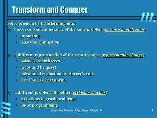
Transform and Conquer • In a transformation stage, modify the problem to make it more amenable to solution • In a conquering stage, solve it • Often employed in mathematical problem solving and complexity theory Simpler Instance OR Another Representation OR Another Problem’s Instance Problem’s Solution Problem’s Instance
Flavours of Transform and Conquer • Instance Simplification = a more convenient instance of the same problem • Presorting • Gaussian elimination • Representation Change = a different representation of the same instance • Balanced search trees • Heaps and heapsort • Polynomial evaluation by Horner’s rule • Problem Reduction = a different problem altogether • Reductions to graph problems
Presorting: Instance Simplification • Solve instance of problem by preprocessing the problem to transform it into another simpler/easier instance of the same problem • Many problems involving lists are easier when list is sorted: • Searching • Computing the median (selection problem) • Computing the mode • Finding repeated elements • Convex Hull and Closest Pair • Efficiency: • Introduce the overhead of an (n log n) preprocess • But the sorted problem often improves by at least one base efficiency class over the unsorted problem (e.g., (n2) (n))
Example: Presorted Selection • Find the kth smallest element in A[1],…, A[n] • Special cases: • Minimum: k = 1 • Maximum: k = n • Median: k = n/2 • Presorting-based algorithm: Sort list Return A[k] • Partition-based algorithm (Variable Decrease & Conquer): Pivot/split at A[s] using Partitioning algorithm from Quicksort IF s=k RETURN A[s] ELSE IF s<k repeat with sublist A[s+1],…A[n] ELSE IF s>k repeat with sublist A[1],…A[s-1]
Notes on the Selection Problem • Presorting-based algorithm: • (n lgn) + (1) = (n lgn) • Partition-based algorithm (Variable decrease & conquer): • Worst case: T(n) =T(n-1) + (n+1) (n2) • Best case: (n) • Average case: T(n) =T(n/2) + (n+1) (n) • Also identifies the k smallest elements (not just the kth) • Simpler linear (brute force) algorithm is better in the case of max & min • Conclusion: Presorting does not help in this case
Finding Repeated Elements • Presorting algorithm for finding duplicated elements in a list: • use mergesort: (n lgn) • scan to find repeated adjacent elements: (n) • Brute force algorithm: • Compare each element to every other: (n2) • Conclusion: presorting yields significant improvement • Similar improvement for mode • What about searching? What about amortised searching? (n lgn)
Balancing Trees • Searching, insertion and deletion in a Binary Search Tree: • Balanced = (log n) • Unbalanced = (n) • Must somehow enforce balance • Instance Simplification: • AVL and Red-black trees constrain imbalances by restructuring trees using rotations • Representation Change: • 2-3 Trees and B-Trees attain perfect balance by allowing more than one element in a node
Heapsort: Representation Change • A heap is a binary tree with the following conditions: • It is essentially complete • The key at each node is ≥ keys at its children • The root has the largest key • The subtree rooted at any node of a heap is also a heap • Heapsort Algorithm: • Build heap • Remove root – exchange with last (rightmost) leaf • Fix up heap (excluding last leaf) • Repeat 2, 3 until heap contains just one node • Efficiency: • (n) + (n log n) = (n log n) in both worst and average cases • Unlike Mergesort it is in place
Horner’s Rule: Representation Change • Addresses the problem of evaluating a polynomial p(x) = an xn + an-1 xn-1 + … + a1x + a0 at a given point x = x0 • Re-invented by W. Horner in early 19th Century • Approach: Convert to p(x) = (… (an x + an-1 ) x + …) x + a0 • Algorithm: • Example: • Q(x) = 2x3 - x2 - 6x + 5 at x = 3 • P[ ]: 2 -1 -6 5 • p: 2 3*2 + (-1) = 5 3*5 + (-6) = 9 3*9 + 5 = 32 p P[n] FOR i n -1 DOWNTO 0 DO p x p + P[i] RETURN p
Notes on Horner’s Rule • Efficiency: • Brute Force = (n2) • Transform and Conquer = (n) • Has useful side effects: • Intermediate results are coefficients of the quotient of p(x) divided by x - x0 • An optimal algorithm (if no preprocessing of coefficients allowed) • Binary exponentiation: • Also uses ideas of representation change to calculate an by considering the binary representation of n
Problem Reduction • If you need to solve a problem reduce it to another problem that you know how to solve • Used in Complexity Theory to classify problems • Computing the Least Common Multiple: • The LCM of two positive integers m and n is the smallest integer divisible by both m and n • Problem Reduction: LCM(m, n) = m * n / GCD(m, n) • Example: LCM(24, 60) = 1440 / 12 = 120 • Reduction of Optimization Problems: • Maximization problems seek to find a function’s maximum. Conversely, minimization seeks to find the minimum • Can reduce between: min f(x) = - max [ - f(x) ]
Reduction to Graph Problems • Algorithms such as Breadth First and Depth First Traversal available after reduction to a graph rep • State-Space Graphs: • Vertices represent states and edges represent valid transitions between states • Often with an initial and goal vertex • Widely used in AI • Example: The River Crossing Puzzle [(P)easant, (w)olf, (g)oat, (c)abbage] Pwgc | | Pwc | | g Pgc | | w Pwg | | c Pg | | wc wc | | Pg c | | Pwg w | | Pgc g | | Pwc | | Pwgc
Strengths and Weaknesses of Transform-and-Conquer • Strengths: • Allows powerful data structures to be applied • Effective in Complexity Theory • Weaknesses: • Can be difficult to derive (especially reduction)