Download
1 / 44
450 likes | 578 Views
NIR Spectroscopy: From PCA to Regression Following the Guiding Discipline . Rodolfo J. Romañach , Ph.D. UPR- Mayagüez rromanac@yahoo.com August 19, 2012. . Begin with the End in Mind – View from 30,000 feet.

E N D
NIR Spectroscopy: From PCA to RegressionFollowing the Guiding Discipline Rodolfo J. Romañach, Ph.D. UPR-Mayagüez rromanac@yahoo.com August 19, 2012.
Begin with the End in Mind – View from 30,000 feet • There are many aspects in this work. Powder samples, tablets, production equipment and the NIR instruments used to obtain spectra and monitor a process. • Software like SIMCA, Unscrambler, Pirouette, PLS Tool Box, PLS IQ, etc that facilitate the careful observation of spectra (or other patterns) studying & understanding the data and then developing the calibration model. • A number of companies sell software for real time predictions. Software that enable the use of the regression equation in the production environment. This is another software that is just for “use” of the calibration model and provide the information to a distributed control system or plant manufacturing data system. • Software for production that control all production systems, including real time predictions, and pickup all the data (e.g. SIPAT, SynTQ, etc.)
The radiation that comes back to the entry surface is called diffuse reflectance. Scattering and Diffuse Reflectance • Light propagates by scattering. • As light propagates, remittance, transmission and absorption occur.
Diffuse Reflectance Reflectance is termed diffuse where the angle of reflected light is independent of the incident angle Spectra Affected by: • Particle size of sample. • Packing density of sample, and pressure on sample. • Refractive index of sample. • Crystalline form of sample. • Absorption coefficients of sample. • Characteristics of the sample’s surface. J.M. Chalmers and G. Dent, “Industrial Analysis with Vibrational Spectroscopy”, Royal Society of Chemistry, 1997, pages 153 -162.
Particle Size and Scattering Smaller particle sizes More remission, less transmission Absorbing power (absence of scattering) Absorption coefficient (includes effects of voids, surface reflection, distance traveled) Larger particle sizes Less remission, more transmission
Additive Scatter Component Only a fraction (1/c) of the remitted light is detected for a particular sample. I detected = 1/c x Iremitted Adetected= - log (Rdetected) = - log (Idetected/I0) = log c + log (I0/Iremitted) = c’ + A If c’ = log (c) is sample dependent, this will cause an additive baseline difference between the samples, i.e. an additive effect in the absorbance values. Naes, Isaksson, Fearn, and Davis, Multivariate Calibration and Classification, page 106- 107, NIR Publications, 2002.
Analytical methods provide information • In NIR spectroscopy this information can be physical or chemical. • If we are not careful we can confuse the two. • Differences in baseline will interfere, with chemical observations, such as drug or water concentration. • Differences in baseline may be removed with pretreatment methods such as first and second derivative.
Differences in Baseline and Slope of Spectra Joshua León, Undergraduate Research, Aug. – Dec. 2008
1st and 2nd Derivative Spectra Remember derivatives indicate change, so a number of changes in spectra may become more evident. Joshua León, Undergraduate Research, Aug. – Dec. 2008
2nd Derivative, 5 Points Segment Original Spectrum Observe the derivatives carefully afternoon performing, working with a low # of points will highlight high frequency noise. 2nd D- 5 points segment
2ndDer., 25 Points Segment Original Spectrum 2nd D- 25 points segment
“Chemometrics is a chemical discipline that uses mathematics, statistics and formal logic a) to design or select optimal performance experimental procedures. b) To provide maximum relevant chemical information by analyzing chemical data. c) To obtain knowledge about chemical systems” Chemometrics Handbook of Chemometrics and Qualimetrics: Part A. D.L. Massart, et. Al. Elsevier, 1997, page 1.
Chemometrics • A = - log I/I0 = - log T. • pH = - log [H+] Simple examples of chemometrics since it helps to visualize data. • May be used for qualitative analysis such as identification testing. Comparison of patterns. • Used for quantitative methods such as drug content in a tablet.
Current Univariate Methods • HPLC used for a large number of analysis. • Only one signal used (absorbance at one wavelength) • A significant amount of time and solvent employed to separate everything and obtain only one component to be measured by the detector.
The Power of Multivariate Analysis Based on Figure 5.2, page 184. Beebe, Pell, Seasholtz, Chemometrics a Practical Guide), Wiley, 1998.
0856 0855 Difficult to see the differences between the two
The Chemometric Approach First, establish a purpose • Simple Understanding: Exploratory Analysis (look at the data, carefully examine it, get a simple visual idea about the main relationships between samples. Chromatogram may contain hundreds of peaks – but the human eye cannot tell those that vary the most from sample to sample Learn • Property Prediction: regression modeling. Compare spectra or patterns. Model • Automate Routine Predictions: if modeling succeeds. Use Infometrix, Chemometrics Training Course, 2004, R.G. Brereton, Chemometrics Data Analysis for the Laboratory and Chemical Plant, Wiley, 2003, page 183.
Working with Variation Patterns Spectrum, A = f(λ), A = f(ν) Chromatogram Area = f(tr) Mass Spectra, Intensity = f(m)/e) Many of the detector responses that we know are patterns of variation, that may be compared. May compare one variable or multiple variables.
Spectra in Spreadsheet Format Row vector, x = [ x1 x2 …., xm] x1 x2xm are called elements of vector. Row vector x = [0.090334 0.091461 0.092569 0.093737] Each row vector applies to a different sample.
Spectrum is a Variation Pattern (function) Interpolation between the different responses provides the spectrum, much like a connect the dots drawing.
Orthogonal Projection The orthogonal projection u of a vector x on another vector y is shown in Fig. 9.4. u = projx = ║x║ycosθ ║y║ Orthogonalization. Vector x is decomposed in two orthogonal (uncorrelated) vectors u and v; u is the orthogonal projection of x on y and v is the vector orthogonal to y. Figure 9.4 Handbook.
Corr. Coeff. For x & y is: 0.9982 Could visualize in terms of two orthogonal vectors. A first that is equivalent to the line y = 1.9818 x + 0.2727, and a second that explains the rest of the variation (residuals).
Alignment of Data Yalignedmay be obtained by subtracting from y the value of the least squares regression, y = = 1.9818 x + 0.2727. The correlation between x and x is now – 0.000618.
X = X’ = TkLkTThe columns of L are the principal components, the new factors or linear combinations of the original variables. PCA – Score Plot Residuals express the remaining or unexplained variation. PC2 PC1 drawn along the axis with > variation of the data PC1 = a11X1 + a12X2 + … + aipXpbased on linear combination of original variables. Residual Score T (scores) co-ordinates in the new axis P (loadings) cosines of new angles with original axes PC1 Projections from the original x1 x2 space on PC1 are called the scores of the objects on PC1.
Same Information Fewer No. Of Original Variables Reduction of Variables 0,02 Principal Component Analysis 0,01 Score PC2 X = T P t + E 0,00 X is Matrix of Spectra -0,01 T (scores) co-ordinates in the new axis P (loadings) cosines of new angles with original axes -0,02 -0,04 -0,03 -0,02 -0,01 0,00 0,01 0,02 0,03 Score PC1 Synthetic samples Doped Samples Production Samples • Provides differentiation of samples. Developed Manel Alcalà, Ph.D.
Principal Components Analysis (PCA) • PCA is built on the assumption that variation implies information. Spectra are variation patterns. • The first PC is the direction through the data that explains the most variability in the data. • The second at subsequent PC’s are orthogonal (at right angles) to the first PC and explain the remaining variation. • The values of individual samples can now be expressed in terms of the PCs as linear summations of the original data multiplied by a coefficient (score). Multivariate Data Analysis, Version 3.11, Infometrix, available from www.infometrix. com
Advantage of PCA Scores in Understanding a Granulation Process J. Rantanen, H. Wikström, R. Turner, and L.S. Taylor, “Use of In-Line Near-Infrared Spectroscopy in Combination with Chemometrics for Improved Understanding of Pharmaceutical Processes, Anal. Chem., 2005, 77, 556 – 563.
Latent Variables • A PC is a latent variable. • This means that the variable is not manifest, it cannot be measured directly. • The latent variables are computed as linear combinations of a set of manifest input variables. • They are called principal because they are particularly dominant or relevant. H. Martens and M. Martens, Multivariate Analysis of Quality, An Introduction. John Wiley & Sons, page 93.
Spectra, PCA Scores Plot, (without pre-treatment) What changes do you see in the spectra ? What is the main source of variation in the spectra ?
After Pre-Treatment of Spectra After pretreatment – in this case SNV-1st-11, the first PC marks the changes in concentration.
PCA Scores Plot A.U. Vanarase, M. Alcalà, J.I. Jerez Rozo, F.J. Muzzio and R.J. Romañach, “Real-time monitoring of drug concentration in a continuous powder mixing process using NIR spectroscopy, Chemical Engineering Science, 2010, 65(21), 5728 – 5733.
Monitoring of Ribbon Density During Roller Compaction. PCA Model Developed with ribbons compacted from 30 – 35 bar. D. Acevedo et.al., AAPSPharmscitech, DOI: 10.1208/s12249-012-9825-0.
A second look at the Math X = X’ = TkLkTThe columns of L are the principal components, the new factors or linear combinations of the original variables which are described in X. T are the scores or weights, and the loadings are the linear combinations of the original variables. The product of TkLkT summarizes the spectral variation observed in X but with orthogonal components. The k refers to the number of vectors or pc’s that will be used to summarize the variation.
PCA – Orthogonality Obtained for spectra from previous slide. Notice that first factor summarizes most of the variation, and then it starts decreasing. Each factor summarizes new variation, not included in previous factors. Pretreatment was not used, only mean centering.
Principal Components Analysis (PCA) • If you know that spectral noise is about 0.1%, then how many • principal components should be used to explain the data ? • Here we have the opportunity to filter or reduce the spectral • noise since we do not have to keep the eight factors.
PCA Scores Plot- The Transition from Qualitative to Quantative A.U. Vanarase, M. Alcalà, J.I. Jerez Rozo, F.J. Muzzio and R.J. Romañach, “Real-time monitoring of drug concentration in a continuous powder mixing process using NIR spectroscopy, Chemical Engineering Science, 2010, 65(21), 5728 – 5733.
Calibration Concepts Calibration requires a training or calibration set (standards) containing measurement of known samples used to prepare the calibration model. The samples in the calibration set should be as representative as possible of all of the unknown samples, which the calibration is expected to successfully analyze. Projection to the Future Reference Method - Standard method that is designated or widely acknowledged as having the highest qualities and whose value is accepted without reference to other standards. Secondary Method - Method whose value is assigned by comparison with a primary standard of the same quality.
Use of PCA to Evaluate Whether Calibration Samples are Representative of Production Samples Comparing the Calibration (highlighted) and Prediction (empty quadrangles) set samples. Calibration – projection to the future.
Developing a Calibration Model • Most NIR calibration models are multivariate. The absorbance at multiple wavelengths or frequencies are mathematically related to an analyte concentration or physical property. • Multivariate regression models like MLR, PLS are used, unlike the univariate linear least squares method used in most analytical chemistry.
O-H first overtone Variation Implies Information !! However, variation could come from differences in moisture content (chemical info) or variation in particle size, porosity, density (physical info). Absorbance, 1st-derivative, and 2nd derivative spectra. X. Zhou, P. Hines, and M.W. Borer, “Moisture Determination in a Hygroscopic drug Substance by Near Infrared Spectroscopy”, Journal of Pharmaceutical and Biomedical Analysis, 17(1998), 219-225.
O-H combination band X. Zhou, P. Hines, and M.W. Borer, “Moisture Determination in a Hygroscopic drug Substance by Near Infrared Spectroscopy”, Journal of Pharmaceutical and Biomedical Analysis, 17(1998), 219-225. Absorbance, 1st-derivative, & 2nd derivative spectra.
Evaluation of pretreatment and spectral area for quantitative method Evaluation of pretreatment and spectral area for quantitative method – C. Peroza Meza, M.A. Santos, and R.J. Romañach, “Quantitation of drug content in a low dosage formulation by Transmission Near Infrared Spectroscopy”, 2006, 7(1), Article 29 (http://www.aapspharmscitech.org).
Begin with the End in Mind – View from 30,000 feet • There are many aspects in this work. Powder samples, tablets, production equipment and the NIR instruments used to obtain spectra and monitor a process. • Software like SIMCA, Unscrambler, Pirouette, PLS Tool Box, PLS IQ, etc that facilitate the careful observation of spectra (or other patterns) studying & understanding the data and then developing the calibration model. • A number of companies sell software for real time predictions. Software that enable the use of the regression equation in the production environment. This is another software that is just for “use” of the calibration model and provide the information to a distributed control system or plant manufacturing data system. • Software for production that control all production systems, including real time predictions, and pickup all the data (e.g. SIPAT, SynTQ, etc.)