Download
1 / 39
390 likes | 539 Views
Physical and Mathematical Interpretations of an Adjoint Model with Application to ROMS. Andy Moore University of Colorado Boulder. Linearized Systems. Consider a state-space (the ocean) with state vectors Denote ROMS is just a set of operators:. In general will be nonlinear.

E N D
Physical and Mathematical Interpretations of an Adjoint Model with Application to ROMS Andy Moore University of Colorado Boulder
Linearized Systems • Consider a state-space (the ocean) with state vectors • Denote • ROMS is just a set of operators: • In general will be nonlinear. • For many problems it is of considerable theoretical and practical interest to consider perturbations to
Let • In which case: • For many problems, it is sufficient to consider small perturbations: and negligible • The Tangent Linear Equation (TLE): • TLE forms core of many analyses (e.g. normal modes, linear iteration of nonlinear problems (data assimil))
Matrix-Vector Notation • ROMS solves the primitive equations in discrete form: NLROMS trajectory
Important Questions • Now that we have reduced the linearized ROMS (TLROMS) to a matrix, what would we like to know? • We should perhaps ask of what value is since in reality ROMS (and the real ocean) is nonlinear?
Justification for TLROMS • All perturbations begin in the linear regime. • Linear regime often continues to provide useful information long after nonlinearity becomes important. • Since the action of is to merely “scatter” energy, linear regime yields stochastic paradigms.
The Propagator • It is more convenient to work in terms of the TLROMS propagator: • So, what would we like to know about ?
Dimension • The ocean is a very large and potentially very complicated place! • But just how complicated is it? • What is it’s effective dimension? • Low dimension described by just a few d.o.f? or high dimension? • Does dimension depend on where we look?
R is BIG!!! • R is a monster! • Can we reduce R to something more managable?
Enter the Adjoint! • Eckart-Schmidt-Mirsky theorem: the most efficient representation of a matrix: where and are the orthonormal singular vectors of • Singular Value Decomposition (SVD).
By definition: where = singular values = transpose propagator or adjoint (wrt Euclidean norm) • Clearly:
Consider: • So looks like an EOF (i.e. something that we “observe”).
The Question of Dimension • The dimension of is equal to the “range” of (i.e. the set of singular vectors with ). • Dimension=“rank”=maximal # of independent rows and columns of • SVD is the most reliable method for determining numerically the rank of a matrix.
Hypothesis • In the limit to its continuous counterpart. • The rank of will provide fundamental information about the dimensionality of the real ocean circulation
The Active and Null Space • i.e. Transforms from v-space to u-space Initial state Final/Observed state • Suppose is an (NxN) matrix of rank P (i.e. ) • If , (i.e. nothing is observed). • is the Null Space of • is the Activated Space of
Null Space Activated Space
Recall: • transforms from “observed u” back to “activated v-space”. • So if we observe “u” the adjoint tells us from whence it came! (cf Green’s functions). Observed State Initial State
Generating Vectors • Let be an (NxM) matrix, where N<M. • SVD yields two fundamental spaces: N-space and M-space M-space to N-space N-space to M-space
Consider the underdetermined system , given; unknown. • Unique solutions exist if: • Then: • is called the “generating vector”. • is called the “natural solution”.
Suppose that has only P non-zero singular values: • SVD: • So is ALWAYS in P-space (i.e. “activated space” identified by )
A Familiar Example • The QG barotropic vorticity equation: • Solve for : underdetermined! • Adjoint vorticity equation yields the generating (stream) function:
Adjoint Applications • Clearly the adjoint operator of ROMS yields information about the subspace or dimensions that are activated by . • There are many applications that take advantage of this important property.
Sensitivity Analysis • Consider a function • Clearly • But • So Sensitivity
Clearly the action of the adjoint restricts the sensitivity analysis to the subspace activated by (i.e. to the space occupied by “natural” solutions).
Least-Squares Fittingand Data Assimilation • If then the gradient provided by can be used to find that minimizes . • The is the idea behind 4-dimensional variational data assimilation (4DVAR) • Clearly the that minimizes lies within the active subspace of
Traditional Eigenmode Analysis • We are often taught to use the eigenmodes of to explore properties and stability of ocean. • In general, the eigenmodes of are NOT orthogonal, meaning each mode has a non-zero projection on other modes. • What does this do to our notion of active and null space?
Null Space based on modes of The two spaces overlap! Activated Space based on modes of
The amplitude of a particular eigenmode of is determined by its projection on the active subspace (i.e. by it’s projection on the corresponding eigenmode of ).
Basin Modes in a Mean Flow Adjoint Eigenmode #6 Eigenmode #6 Basic State Circulation
SVD and Generalized StabilityAnalysis • Recall from SVD that: • Time evolved SV is • Ratio of final to initial “energy” is: • So of all perturbations, is the one that maximizes the growth of “energy” over the time interval .
Consider the forced TL equation: • If is stochastic in time, more general forms of SVD are of interest. • Assume unitary forcing: • Of particular interest are: Controllability Grammiam Observability Grammiam
Eigenvectors of are the EOFs. • Eigenvectors of are the Stochastic Optimals. • Variance: • Eigenvectors of are balanced truncation vectors. • All have considerable practical utility and applications that go far beyond traditional eigenmode analysis!
Covariance Functions andRepresenters • The “controllability” Grammiam is nothing more than a covariance matrix. • Note that looks a lot like: which yields the “natural solution”. • Operations involving yield only natural solutions related to “Representer Functions”.
Norm Dependence • The adjoint is norm dependent. • For the Euclidean norm, • Changing norms is simply equivalent to a rotation and/or change in metric Null Space Activated Subspace
Summary Null Space The adjoint identifies the bits of state-space that actually do something! Activated Space
The Adjoint of ROMS is a Wonderful Thing!
The Cast of Characters - played by NLROMS - played by TLROMS - played by ADROMS
Acknowledgements • Lanczos, C., 1961: Linear Differential Operators, Dover Press. • Klema, V.C. and A.J. Laub, 1980: The Singular Value Decomposition: Its Computation and Some Applications. IEEE Trans. Automatic Control, AC-25, 164-176. • Wunsch, C., 1996: The Ocean Circulation Inverse Problem, Cambridge University Press. • Brogan, W.L., 1991: Modern Control Theory, Prentice Hall. • Bennett, A.F., 1992: Inverse Methods in Physical Oceanography, Cambridge University Press. • Bennett, A.F., 2002: Inverse Modeling of the Ocean and Atmosphere, Cambridge University Press. • Benner, P., P. Mehrmann and D. Sorensen, 2005: Dimension Reduction of Large-Scale Systems. Lecture Notes in Computational Science and Engineering, Vol. 45, Springer-Verlag. • Trefethen, L.N and M. Embree, 2005: Spectra and Pseudospectra, Princeton University Press. • Farrell, B.F. and P.J. Ioannou, 1996: Generalized Stability Theory, Part I: Autonomous Operators. J. Atmos. Sci., 53, 2025-2040. • Farrell, B.F. and P.J. Ioannou, 1996: Generalized Stability Theory, Part II: Nonautonomous Operators. J. Atmos. Sci., 53, 2041-2053.
R is BIG!!! • R is a monster! • Can we reduce R to something more managable?