Download
1 / 18
180 likes | 286 Views
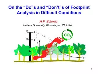
H.P. Schmid. Indiana University, Bloomington IN, USA. CO 2. ?. On the “Do”s and “Don’t”s of Footprint Analysis in Difficult Conditions. The earliest documented footprint-type idea:. The “Effective Fetch” of Frank Pasquill (1972).

E N D
H.P. Schmid Indiana University, Bloomington IN, USA CO2 ? On the “Do”s and “Don’t”s of Footprint Analysis in Difficult Conditions
The earliest documentedfootprint-typeidea: The “Effective Fetch” of Frank Pasquill (1972) Pasquill, F.: 1972. 'Some aspects of boundary layer description'. Q. J. R. Meteorol. Soc., 98, 469-494. Frank Pasquill, FRS1914 - 1994
Effective fetch isopleths (C/Cmax = ½) dependent on height, stability and roughness
applicability complexity In the time since Pasquill: Several Types of Footprint Models • Analytical • Stochastic (Lagrangian) • Closure Models • Large-Eddy Simulation • For reviews of individual models, see: • Schmid, Ag.For.Met., 113, 2002: 159-183. • Foken & Leclerc, Ag.For.Met, 127, 2004: 223-234.
Flux Footprint = spatial filter, “field of view” (convolution of the source distribution,QS, with the footprint,f ) : scalar flux, F; or scalar concentration, c
: surface sources flux production rate(arises from c-gradient in turbulent flow). surface sources only in boundary conditions Concentration and Flux Footprint Models Governing equations in Eulerian analysis:* advection diffusion forcing F: in inhomogeneous flow, may cause complex behavior of flux footprint * following Finnigan (2004, AgForMet 127, 117-129); neglecting horizontal turbulent fluxes and pressure interactions.
solution for crosswind integrated concentration, Analytical Footprint Models Aad van Ulden (1978): Realistic analytic solution of advection-diffusion equation: • based on power-law profiles • fitting power-laws to similarity profiles • M-O scaling widely used for analytic source area and footprint models (with some exceptions!) Van Ulden, A.P., 1978. ‘Simple estimates for vertical diffusion from sources near the ground’, Atmos. Environ., 12, 2125-2129.
based on theLangevin Equation: correlated part particlevelocity random part Flux Distribution Lagrangian Stochastic Footprint Models Joseph-Louis Lagrange (1736-1813) Paul Langevin(1872-1946) • need large number of particles • need flow and turbulence • adaptable to vertically inhomogeneous turbulence (e.g., forest canopies) Continuous Point Source
Forest Canopy LS-Footprint Models Dennis D. Baldocchi* • forward well-mixed LS model (2-D, 3D) • parameterized turbulence/flow profiles • vertically inhomogeneous turbulence • includes streamwise diffusion * Baldocchi, D.D., Ag. For. Met. 85, 1997: 273-292.
by the Inverse Plume Assumption flux plume from surface point source inverted plume from virtual source wind virtualwind Projected Footprint Usage of Analytical & (forward) LS-Models • motivated by spatial inhomogeneity (in the scalar field) • assume horizontal homogeneity (in flow and turbulence) invalid ! Point Source Virtual Source
Alternatives for Inhomogeneous Flow Footprint computation based on full (Eulerian) flow models (plus scalar transport equation or LS-module): Claude Louis Marie Henri Navier (1785-1836) • Closure Models • LES Models George Gabriel Stokes (1819-1903) Depending on resolution and closure / sub-grid scale treatment: James W. Deardorff (born 1928) • can be made applicableto any complex condition • can be computationally very intensive Monique Y.Leclerc (born...not long ago) These models are not footprint models per se, but full flow models used to compute a footprint.
Alternatives for Inhomogeneous Flow • Backward LS-Model applicable in principle, but has never been done to date Sensor: continuous “backward release” point Direct Footprint “Touchdown” Source Locations • no Inverse Plume Assumption needed • applicable in weakly inhomogeneous canopies
Objective: Examine Applicability of Footprint Model Types in “Difficult Conditions” “Difficult Conditions” ??? deviations from micrometeorological ideal: • flat terrain • homogeneous fetch • low, homogeneous vegetation (if any) • stationarity • well-developed turbulence (MOST) • topography • patchy land-cover • deep, multy-layer vegetation canopy • instationarity • weak turbulence; free convection
Thou must provide flux data ! Flux Measurement in Difficult Conditions and Footprint Modeling in Difficult Conditions Micrometeorologist’s traditional knee-jerk reaction: Stay away from it!
Difficult Conditions: Patchy Land Cover HeterogeneousScalar Field (DLAI, DBowen-Ratio) • “non-difficult” condition • any footprint model applies • analytic models have restriction to MOST HeterogeneousFlow/Turbulence (disturbance, forest edges) • “inverse plume assumption” (analytical, forward LS) does not apply • full flow model needed • case poorly understood
Difficult Conditions: Deep Canopies Tall Trees • analytical models apply only if zm > 2h (Rannik et al. 2000) • “forest” model better • sensitive to turbulence profiles • “forest” model needed • sensitive to turbulence profiles • “inverse plume assumption” (horizontal homogeneity) questionable Multi-Layer Understorey
Difficult Conditions: Topography Large Scale Topography • use footprint model only (with caution!) for small zm/h: local footprint • use footprint model only for qualitative analysis • full flow model is preferred Small Scale, Gentle Topography • use footprint model if terrain following flow can be assumed (stable conditions?) • “inverse plume assumption”??? • use footprint model only for qualitative analysis
10 The Footprint Modeling Commandments • Know the site! • Know the model! • Know the assumptions! • Thou shall not use a model outside its applicability range! • Thou shall not call it “footprint” if the model does not use unit source strength! • Thou shall not invert a footprint model to estimate a flux! • Thou shall not use a scalar footprint model for non-scalars! • Thou shall exercise caution when using a footprint model with non-passive scalars! • Thou shall never blindly believe any footprint model result, but examine it in the context of the site (see I.)! • Thou shall not complain that there are only nine commandments!