Download
1 / 39
400 likes | 530 Views
Atmospheric carbon-14 as a tracer of the contemporary carbon cycle. Nir Y Krakauer NOAA Climate and Global Change Postdoctoral Fellow Department of Earth and Planetary Science University of California at Berkeley niryk@berkeley.edu. The atmospheric CO 2 mixing ratio.

E N D
Atmospheric carbon-14 as a tracer of the contemporary carbon cycle Nir Y Krakauer NOAA Climate and Global Change Postdoctoral Fellow Department of Earth and Planetary Science University of California at Berkeley niryk@berkeley.edu
The atmospheric CO2 mixing ratio Australian Bureau of Meteorology
Outstanding Questions • Only half of the CO2 produced by human activities is remaining in the atmosphere • Where are the sinks that are absorbing over 40% of the CO2 that we emit? • Land or ocean? • Tropics/Midlatitudes? • Why does CO2 buildup vary dramatically with nearly uniform emissions? • How will CO2 sinks respond to climate change?
Inversions for CO2 sources/sinks Inversion: To fit observations of atmospheric CO2 concentration, seek the optimal combination of regional sources/sinks {mk}:minimize J = Sstn {[ Cobs(stn) – Skmkck (stn)] 2 / sstn2} +Sk{[ mk – mkprior]2 / lk2} + .. • Obs. Network – • mainly remote marine locations • Trying to infer information over land • Under-determined; non-unique solutions; prior estimates of source/sinks as additional constraints
Multimodel inversion for carbon sinks (TransCom) • Key points • Assuming a reasonably well-known ocean sink distribution implies a mid-latitude land sink NOW, comparable to ocean sink • Mechanisms unclear • Few (noisy) in-situ atm. obs. over continents • Ecosystems too heterogeneous for extrapolating the few flux measurements from e.g. towers • On the ocean side, the Southern Ocean, where the initial uncertainty was taken to be large, seems to have a smaller sink than expected Gurney et al. Nature 2005
Caltech: thesis work Tracing Recent Carbon Uptake by Oceans and Land Plants • The impact of volcanic eruptions on global tree productivity • Inferring flux patterns from atmosphere CO2 concentrations: An application of generalized cross validation • The regional distribution of air-sea gas exchange • Seasonality in fossil fuel emissions, respiration, and cross-tropopause transport in Δ14C of atmospheric CO2 Pictures: USGS; LTRR; Ruth Brownlee; Photofusion (via the UK Science Museum)
Berkeley: water-plant-climate interactionswarming, drought and future biotic carbon uptake The Keck Hydrowatch Project:water’s ‘life-cycle’ in California forests • Measurement program to include ~500 solar-powered motes under, on and atop trees organized as wireless networks to measure temperature, humidity, radiation, soil moisture, sap flow • Use to improve representation of land-surface (soil, plant, groundwater) processes in models of hydrology and mesoscale circulation P. Dutta; Arora et al 2005
Ocean CO2 uptake • The ocean must be responding to the higher atmospheric pCO2; models estimate ~2 Pg C/ year uptake • Actual uptake pattern is inferred from measurements of sea-surface pCO2 + estimates of the gas transfer velocity • Bulk parameterization of gas exchange: F = kw (Cs – Ca) • F: gas flux (mass per surface area per time) • Cs: gas concentration in bulk water (mass per volume) • Ca: gas concentration in bulk air (partial pressure * solubility) • kw: gas transfer coefficient (a “gas transfer velocity”) LDEO
Physical models of air-sea gas exchange • Stagnant film model: Air-sea gas exchange is limited by diffusion across a thin (<0.1 mm) water-side surface layer; more turbulent energy thinner layer • Surface renewal model: the surface layer is periodically replaced by new water from below; more turbulent energy more frequent renewal • The air-sea interface becomes complicated (sea spray, bubbles), and physically poorly understood, in stormy seas 100 μm J. Boucher, Maine Maritime Academy
Measured gas transfer velocities range widely… • Gas transfer velocity usually plotted against windspeed (roughly correlates w/ surface turbulence) • Many other variables known/theorized to be important: wave development, surfactants, rain, air-sea temperature gradient… • Several measurement techniques have been used (tracer release, eddy covariance, …) – all imprecise, sometimes seem to give systematically different results Wu 1996; Pictures: WHOI • What’s a good mean transfer velocity to use?
..as do parameterizations of kw versus windspeed • Common parameterizations assume kw to increase with windspeed v (piecewise) linearly (Liss & Merlivat 1986), quadratically (Wanninkhof 1992) or cubically (Wanninkhof & McGillis 1999) • Large differences in implied kw, particularly at high windspeeds (where there are few measurements) • My approach: Are these formulations consistent with ocean tracer distributions? Feely et al 2001
Windspeed varies by latitude Climatological windspeed estimated from satellite measurements (SSM/I; Boutin and Etcheto 1996)
The air-sea CO2 flux is also of different sign at high vs. low windspeed regions • Sea-surface pCO2 is high in the tropics (→ flux out of ocean) and low in the midlatitudes (→ flux into ocean) Takahashi et al 2002
CO2 isotope gradients are excellent tracers of air-sea gas exchange • Because most (99%) of ocean carbon is ionic and doesn’t directly exchange, CO2 air-sea gas exchange is slow to restore isotopic equilibrium • Thus, the size of isotope disequilibria is uniquely sensitive to the gas transfer velocity kw ppm Sample equilibration times with the atmosphere of a perturbation in tracer concentration for a 50-m mixed layer μmol/kg Ocean carbonate speciation(Feely et al 2001)
The radiocarbon (14C) cycle at steady state • 14C (λ1/2 = 5730 years) is produced in the upper atmosphere at ~6 kg / year • Notation: Δ14C = 14C/12C ratio relative to the preindustrial troposphere Stratosphere+80‰ 90 Pg C 14N(n,p)14C Troposphere0‰ 500 Pg C Land biota–3‰ 1500 Pg C Air-sea gas exchange Shallow ocean –50‰ 600 Pg C Deep ocean–170‰ 37000 Pg C Sediments–1000‰ 1000000 Pg C
The bomb spike: atmosphere and surface ocean Δ14C since 1950 • Massive production in nuclear tests ca. 1960 (“bomb 14C”) • Through air-sea gas exchange, the ocean took up ~half of the bomb 14C by the 1980s data: Levin & Kromer 2004; Manning et al 1990; Druffel 1987; Druffel 1989; Druffel & Griffin 1995 bomb spike
Ocean bomb 14C uptake: previous work • Broecker and Peng (1985; 1986; 1995) used 1970s (GEOSECS) measurements of 14C in the ocean to estimate the global mean transfer velocity, <k>, at 21±3 cm/hr • This value of <k> has been used in most subsequent parameterizations of kw(e.g. Wanninkhof 1992) and for modeling ocean CO2 uptake • Based on trying to add up the bomb 14C budget, suggestions have been made (Hesshaimer et al 1994; Peacock 2004)are that Broecker and Peng overestimated the ocean bomb 14C inventory, so that the actual value of <k> might be lower by ~25%
Ocean 14C goals • From all available (~17,000) ocean Δ14C observations, re-assess the amount of bomb 14C taken up, estimate the global mean gas transfer velocity, and bound how it varies by region • The 1970s (GEOSECS) observations plus measurements from more recent cruises (WOCE) data: Key et al 2004
Modeling ocean bomb-14C uptake • Simulate ocean uptake of bomb 14C (transport fields from ECCO-1°), given the known atmospheric history, as a function of the air-sea gas transfer velocity • Find the air-sea gas transfer velocity that best fits observed14C levels
Optimization scheme Assume that kw scales with some power of climatological windspeed u: kw = <k> (un/<un>) (Sc/660)-1/2, (where <> denotes a global average, and the Schmidt number Sc is included to normalize for differences in gas diffusivity) find the values of <k>, the global mean gas transfer velocity and n, the windspeed dependence exponent that best fit carbon isotope measurements using transport models to relate measured concentrations to corresponding air-sea fluxes
Results: simulated vs. observed bomb 14C by latitude – 1970s • For a given <k>, high n leads to more simulated uptake in the Southern Ocean, and less uptake near the Equator • Observation-based inventories seem to favor low n (i.e. kw increases slowly with windspeed) • 1990s (WOCE) observations are also most compatible with a low value of n Simulations for <k> = 21 cm/h and n = 3, 2, 1 or 0 Observation-based estimates (solid lines) from Broecker et al 1995; Peacock 2004
Simulated-observed ocean 14C misfit as a function of <k> and n • The minimum misfit between simulations and (1970s or 1990s) observations is obtained when <k> is close to 21 cm/hr and n is low (1 or below) • The exact optimum <k> and n change depending on the misfit function formulation used (letters; cost function contours are for the A cases) , but a weak dependence on windspeed (low n) is consistently found
Optimum gas transfer velocities by region • As an alternative to fitting <k> and n globally, I estimated the air-sea gas exchange rate separately for each region, and fit <k> and n based on regional differences in windspeed • Compared with previous parameterizations (solid lines), found that kw is relatively higher in low-windspeed tropical ocean regions and lower in the high-windspeed Southern Ocean (+s and gray bars) • Overall, a roughly linear dependence on windspeed (n ≈ 1; dashed line)
Simulated mid-1970s ocean bomb 14C inventory vs. <k> and n • The total amount taken up depends only weakly on n, so is a good way to estimate <k> • The simulated amount at the optimal <k> (square and error bars) supports the inventory estimated by Broecker and Peng (dashed line and gray shading)
Other evidence: atmospheric Δ14C °N • I estimated latitudinal differences in atmospheric Δ14C for the 1990s, using observed sea-surface Δ14C, biosphere C residence times (CASA), and the atmospheric transport model MATCH • The Δ14C difference between the tropics and the Southern Ocean reflects the effective windpseed dependence (n) of the gas transfer velocity
Observation vs. modeling • The latitudinal gradient in atmospheric Δ14C (dashed line) with the inferred <k> and n, though there are substantial uncertainties in the data and models (gray shading) • More data? (UCI measurements) • Similar results for preindustrial atmospheric Δ14C (from tree rings) • Also found that total ocean 14C uptake preindustrially and in the 1990s is consistent with the inferred <k> <k> (cm/hr) n (‰ difference, 9°N – 54°S)
14C conclusions • The power law relationship with the air-sea gas transfer velocity kw that best matches observations of ocean bomb 14C uptake has • A global mean <k>=20±3 cm/hr, similar to that found by Broecker and Peng • A windspeed dependence n= 0.7±0.4 (about linear), compared with 2-3 for quadratic or cubic dependences • This is consistent with other available 14C measurements
The ocean is now releasing 13C to the atmosphere… 1977-2003 • Notation – δ13C: 13C/12C ratio relative to a carbonate standard • The atmospheric 13C/12C is steadily declining because of the addition of fossil-fuel CO2 with low δ13C; this fossil-fuel CO2 is gradually entering the ocean Scripps (CDIAC)
…and the amount can be estimated… PgC∙‰ carbon-13 • Budget elements • the observed δ13C atmospheric decline rate (arrow 1) • biosphere disequilibrium flux (related to the carbon residence time) (5) • fossil fuel emissions (6) • biosphere (4) and ocean (2) net carbon uptake (apportioned using ocean DIC measurements) • I calculated that air-sea exchange must have brought 70±17 PgC∙‰ 13C to the atmosphere in the mid-1990s, ~half the depletion attributable to fossil fuels Pg carbon Randerson 2004
…but the air-sea δ13C disequilibrium is of opposite sign at low vs. high latitudes Sea-surface δ13C (‰) • Reflects fractionation during photosynthesis + temperature-dependent carbonate system fractionation • The dependence of kw on windspeed must yield the inferred global total flux Air-sea δ13C disequilibrium (‰) data: GLODAP (Key 2004) Temperature-dependent air-sea fractionation (‰)
Simulated 1990s air-sea δ13C flux vs. <k> and n • At high n, the 13C flux into the Southern Ocean largely offsets the 13C flux out of the tropics • The observed rate of decline of atmospheric δ13C, combined with the known fossil fuel emissions, suggests a large 13C flux out of the ocean (dashed line and gray shading), which requires n < 2
Implications for ocean CO2 uptake • We can apply the new parameterization of gas exchange to pCO2 maps: • uptake by the Southern Ocean [high windspeed] is lower than previously calculated (fitting inversion results better) • outgassing near the Equator [low windspeed] is higher (reducing the required tropical land source)
Conclusions • 14C and 13C measurements constrain the mean air-sea gas transfer velocity and its spatial/windspeed dependence, averaged over large regions and several years • The new parameterization promises to increase the usefulness of ocean pCO2 measurements for answering where carbon uptake is occurring and how it changes with time (e.g. tropical land vs. ocean) N. Y. Krakauer, J. T. Randerson, F. W. Primeau, N. Gruber, D. Menemenlis, Tellus (2006)
Work in progress • How do we reconcile bottom-up with top-down estimates (work with COARE gas exchange parameterization)? • Might a polynomial match the relationship of the gas transfer velocity with windspeed better than a power law (e.g. kw is not zero in calm seas)? • Are there other quantities that can be measured remotely, such as mean square surface slope or fractional whitecap coverage, that predict gas transfer velocities better than windspeed? • Does the dependence on windspeed change if we use the same high-resolution winds that drive model ocean mixing?
Acknowledgements • Advisors and collaborators: Jim Randerson, Tapio Schneider, François Primeau, Dimitris Menemenlis, Nicolas Gruber • Δ14C measurements and interpretation: Stanley Tyler, Sue Trumbore, Xiaomei Xu, John Southon, Jess Adkins, Paul Wennberg, Yuk Yung • Inez Fung and the Keck Hydrowatch team • NOAA, NASA, and the Betty and Gordon Moore Foundation for fellowships • The Earth System Modeling Facility for computing support
Warming is underway Dragons Flight (Wikipedia) Data: Hadley Centre
CO2 Inversions: (1) Forward Step • Premise: Atm CO2 = linear combination of response to each source or sink • Divide surface into “basis regions” • Specify unitary source (e.g. 1 PgC/month) each month from each region • Simulate atm CO2 “basis” response with atm general circulation model