Download

1 / 28
280 likes | 592 Views
Loglinear Contingency Table Analysis. Karl L. Wuensch Dept of Psychology East Carolina University. The Data. Weight Cases by Freq. Crosstabs. Cell Statistics. LR Chi-Square. Model Selection Loglinear. HILOGLINEAR happy(1 2) marital(1 3) /CRITERIA ITERATION(20) DELTA(0)

E N D
Loglinear Contingency Table Analysis Karl L. Wuensch Dept of Psychology East Carolina University
Model Selection Loglinear HILOGLINEAR happy(1 2) marital(1 3) /CRITERIA ITERATION(20) DELTA(0) /PRINT=FREQ ASSOCIATION ESTIM /DESIGN. • No cells with count = 0, so no need to add .5 to each cell. • Saturated model = happy, marital, Happy x Marital
The Model Fits the Data Perfectly, Chi-Square = 0 • The smaller the Chi-Square, the better the fit between model and data.
Both One- and Two-Way Effects Are Significant • The LR Chi-Square for Happy x Marital has the same value we got with Crosstabs
The Model: Parameter Mu • LN(cell freq)ij = + i + j + ij • We are predicting natural logs of the cell counts. • is the natural log of the geometric mean of the expected cell frequencies. • For our data, and LN(154.3429) = 5.0392
The Model: Lambda Parameters • LN(cell freq)ij = + i + j + ij • i is the parameter associated with being at level i of the row variable. • There will be (r-1) such parameters for r rows, • And (c-1) lambda parameters, j, for c columns, • And (r-1)(c-1) lambda parameters, for the interaction, ij.
Main Effect of Marital Status • For Marital = 1 (married), = +.397 • for Marital = 2 (single), = ‑.415 • For each effect, the lambda coefficients must sum to zero, so • For Marital = 3 (split), = 0 ‑ (.397 ‑ .415) = .018.
Main Effect of Happy • For Happy = 1 (yes), = +.885 • Accordingly, for Happy =2 (no), is ‑.885.
Happy x Marital • For cell 1,1 (Happy, Married), = +.346 • So for [Unhappy, Married], = -.346 • For cell 1,2 (Happy, Single), = -.111 • So for [Unhappy, Single], = +.111 • For cell 1,3 (Happy, Split), = 0 ‑ (.346 ‑ .111) = ‑.235 • And for [Unhappy, Split], = 0 ‑ (‑.235) = +.235.
Interpreting the Interaction Parameters • For (Happy, Married), = +.346 There are more scores in that cell than would be expected from the marginal counts. • For (Happy, Split), = 0 ‑.235 There are fewer scores in that cell than would be expected from the marginal counts.
Predicting Cell Counts • Married, Happy e(5.0392 + .397 +.885 +.346) = 786 (within rounding error of the actual frequency, 787) • Split, Unhappy e(5.0392 + .018 -.885 +.235) =82, the actual frequency.
Testing the Parameters • The null is that lambda is zero. • Divide by standard error to get a z score. • Every one of our effects has at least one significant parameter. • We really should not drop any of the effects from the model, but, for pedagogical purposes, ………
Drop Happy x Marital From the Model HILOGLINEAR happy(1 2) marital(1 3) /CRITERIA ITERATION(20) DELTA(0) /PRINT=FREQ RESID ASSOCIATION ESTIM /DESIGN happy marital. • Notice that the design statement does not include the interaction term.
Uh-Oh, Big Residuals • A main effects only model does a poor job of predicting the cell counts.
Big Chi-Square = Poor Fit • Notice that the amount by which the Chi-Square increased = the value of Chi-Square we got earlier for the interaction term.
Pairwise Comparisons • Break down the 3 x 2 table into three 2 x 2 tables. • Married folks report being happy significantly more often than do single persons or divorced persons. • The difference between single and divorced persons falls short of statistical significance.
SPSS Loglinear LOGLINEAR Happy(1,2) Marital(1,3) / CRITERIA=Delta(0) / PRINT=DEFAULT ESTIM / DESIGN=Happy Marital Happy by Marital. • Replicates the analysis we just did using Hiloglinear. • More later on the differences between Loglinear and Hiloglinear.
SAS Catmod options pageno=min nodateformdlim='-'; data happy; input Happy Marital count; cards; 1 1 787 1 2 221 1 3 301 2 1 67 2 2 47 2 3 82 proccatmod; weight count; model Happy*Marital = _response_; Loglin Happy|Marital; run;
PASW GENLOG GENLOG happy marital /MODEL=POISSON /PRINT=FREQ DESIGN ESTIM CORR COV /PLOT=NONE /CRITERIA=CIN(95) ITERATE(20) CONVERGE(0.001) DELTA(0) /DESIGN.
GENLOG Coding • Uses dummy coding, not effects coding. • Dummy = One level versus reference level • Effects = One level versus versus grand mean • I don’t like it.
Catmod Output • Parameter estimates same as those with Hilog and loglinear. • For the tests of these paramaters, SAS’ Chi-Square = the square of the z from PASW. • I don’t know how the entries in the ML ANOVA table were computed.