Download
1 / 42
420 likes | 540 Views
VARSY Final Presentation ATLID-CPR-MSI Clouds, Aerosols and Precipitation “Best Estimate”. Robin Hogan, Nicola Pounder, Brian Tse , Chris Westbrook University of Reading. 9 October 2013. Overview. Why do we need ACM-CAP? Example retrieval using A-Train data How does it work?

E N D
VARSY Final PresentationATLID-CPR-MSI Clouds, Aerosols and Precipitation “Best Estimate” Robin Hogan, Nicola Pounder, Brian Tse, Chris Westbrook University of Reading 9 October 2013
Overview • Why do we need ACM-CAP? • Example retrieval using A-Train data • How does it work? • Ice-cloud component • Retrieving the degree of riming • *Impact of realistic ice scattering model • Liquid-cloud component • Rain component • *Coping with non-monotonic forward model • Aerosol component • Kalman smoother • Error reporting • *Including errors in the retrieval assumptions • Remaining work (post VARSY) *Done since last meeting This talk demonstrates concepts using A-Train data, but have successfully tested ACM-CAP on EarthCARE data simulated from A-Train retrievals
Justification for ACM-CAP Why retrieve clouds, aerosols and precipitation together? • Vertically integrated information (e.g. from radiances and path-integrated attenuation) is influenced by multiple atmospheric constituents so can only be interpreted correctly if those constituents are retrieved simultaneously Why combine radar, lidar and radiometer? • Clouds described by at least two variables (e.g. number and size) so at least two measurements needed (e.g. radar and lidar) • Radar and lidar have different sensitivities, so combining them leads to a seamless retrieval • Solar and infrared radiances improve radiative accuracy of retrievals, important for closing the solar and infrared radiation budget • EarthCARE was designed with synergy in mind
What the results look like so far CloudSat observations CloudSat forward model Calipso observations Calipso forward model
Ice extinction coefficient Liquid water content Rain rate Aerosol extinction coefficient
Unified retrieval Ingredients developed Done in VARSY Not yet completed 1. Define state variables to be retrieved (x) Use classification to specify variables describing each species at each gate Ice and snow: extinction coefficient,N0’,lidar ratio, riming factor Liquid: extinction coefficient and number concentration Rain: rain rate, drop diameter and melting ice Aerosol:number concentration, particle size and lidar ratio 2. Forward model 2a. Radar model With multiple scattering, Doppler and PIA 2b. Lidar model Including HSRL channels and multiple scattering 2c. Radiance model Solar & IR channels 4. Iteration method Derive a new state vector: quasi-Newton or Levenberg-Marquardtscheme Not converged 3. Compare to observations (y) Check for convergence Converged 5. Calculate retrieval error Error covariances & averaging kernel Proceed to next ray of data
(2) (2b) (3) (3b) (1) Calculate scattering and absorption of air from T, p, q (4) (5)
Minimizing the cost function Gradient of cost function (a vector) Gauss-Newton method Rapid convergence Levenberg-Marquardt is a small modification to ensure convergence Expensive to compute Jacobian & Hessian • and 2nd derivative (the Hessian matrix): • Quasi-Newton methods • Fast adjoint method to calculate xJ means don’t need to calculate Jacobian • L-BFGS (e.g. used by ECMWF): builds up an approximate inverse Hessian A from multiple gradients xJ • Scales well for large x • Disadvantage: more iterations needed since we don’t know curvature of J(x) Both Levenberg-Marquardt and L-BFGS have been implemented
Flexibility Object-oriented implementation allows great flexibility • The following can be configured easily at run-time • What observations are to be used, and their characteristics • What atmospheric constituents are to be retrieved • What state variables are to be used to describe the constituents • How vertical profile of state variables are to be represented • Easy to apply same algorithm to A-Train, EarthCARE& other platforms Automatic differentiation makes the code easy to develop and extend • Every line of the forward model code needs to be differentiated • Major effort to do this by hand (as done at ECMWF, Met Office etc!) • “Adept” C++ library developed during VARSY (Hogan 2013) • Minimal code changes and differentiation can be automated • Faster than all existing libraries that take the same approach • Nearly as fast as hand-coded adjoint • Jacobian calculation can be parallelized on multi-core machines (looks more promising than GPU)
Ice cloud retrieval: status • State variables similar to those used by Delanoe and Hogan (2008) • Ice extinction • N0’: measure of number conc. with good a priori temperature dependence • Lidar backscatter-to-extinction ratio • Riming factor: scales ice density so Doppler can be used to infer riming • Features • Ice and snow treated as one: snow flux reported for all ice clouds • New “self-similar Rayleigh Gans” model for radar scattering by large ice and snow (two orders of magnitude larger for 1-cm snow than soft spheroid) • Further work • Testing, particularly on datasets with Doppler and radiances
Extending ice retrievals to riming snow • Retrieve a riming factor (0-1) which scales b in mass=aDb between 1.9 (Brown & Francis) and 3 (solid ice) 0.9 0.8 0.7 0.6 • Heymsfield & Westbrook (2010) fall speed vs. mass, size & area • Brown & Francis (1995) ice never falls faster than 1 m/s Brown & Francis (1995)
Examples of snow35 GHz radar at Chilbolton 1 m/s: no riming or very weak 2-3 m/s: riming? • PDF of 15-min-averaged Doppler in snow and ice (usually above a melting layer)
Radar scattering by ice 1 mm ice 1 cm snow • Hogan and Westbrook (2013) used simulated ice aggregates to derive an equation for radar backscatter: the “Self-Similar Rayleigh Gans approximation” • For snowflakes, internal structures on scale of wavelength lead to 1-3 orders of magnitude higher backscatter than “soft spheroids” Realistic aggregate snowflake Soft spheroid
Ice aggregates Ice spheres Impact of ice shape on retrievals • Spheres can lead to overestimate of water content and extinction of factor of 3 • All 94-GHz radar retrievals affected in same way
Liquid cloud retrieval: status • State variables • Liquid water content LWC • Total number concentration (one value per layer, need solar radiances to retrieve it): more likely to be constant with height than effective radius • Features • One-sided gradient constraint prevents LWC variation with height that is steeper than adiabatic: helps extrapolate lidar information to cloud base, improving cloud base height estimate • Capability to exploit lidar multiple scattering for good optical depth retrieval, but less applicable to EarthCARE with small ATLID footprint • Further work • Test impact of solar radiances to retrieve number concentration
Rain retrieval: status • State variables • Rain rate • Normalized number concentration (constant with height, need PIA to retrieve it) • Features • “Flatness” constraint on rain rate penalizes variations with height, so attenuation interpreted in terms of rain rate (e.g. Matrosov 2007) • Future work • Test assimilation of radar PIA as a constraint (e.g. Haynes et al. 2009) • Use PIA to resolve retrieval ambiguity arising from strong attenuation • Test impact of Doppler measurements Melting ice in the melting layer • Currently its radar attenuation is simply parameterized as a function of rain rate (Matrosov 2008) • Can retrieve a scaling factor for this attenuation; could be used if PIA was assimilated
Rain retrieval ambiguity • For an observed Z profile there are often two ways to fit it: • Low rain rate: low attenuation • High rain rate: high attenuation • Retrieval is then dependent on intelligent first guess No attenuation Rayleigh scattering radar 94-GHz radar Attenuation through 500-m of rain 94-GHz radar
Often two different rain profiles can forward model the observed reflectivity profile Over ocean could discriminate between the two with PIA Rain retrieval Low prior (0.01 mm h-1) Default prior (5 mm h-1)
Could EarthCARE do better? • Forward model EarthCARE Doppler in the two scenarios • Velocity different by 1-2 m s-1, even though measured reflectivity is about the same • Hence EarthCARE Doppler will discriminate between these solutions as long as air motion is not too strong Low prior (0.01 mm h-1) Default prior (5 mm h-1)
Aerosol retrieval: status • State variables • Total number concentration • Median volumetric diameter D0 (one value per layer, need solar radiances) • Lidar backscatter-to-extinction ratio (need HSRL) • Features • Kalman smoother has been implemented to provide adaptive smoothing in time • Particle type (and hence refractive index) is prescribed; operationally this would come from an ATLID-only classification • Particles are assumed to be spherical: this could be changed • Further work • Test retrieval of backscatter-to-extinction ratio using real HSRL data • Test impact of solar radiances to retrieve D0 • Kalman smoother is forward only: implement reverse pass so smoothing is symmetric in time
Kalman smoother Splines to smooth vertically Vertical smoothing plus Kalman smoother • ATLID-only aerosol retrievals pre-average lidar due to low signals • Kalman smoother achieves similar effect on profile-by-profile retrieval • Extra term added to cost function penalizing diff. from previous ray • Reverse pass (not yet implemented) ensures this is symmetric in time Calipso back-scatter Retrieved aerosol number conc
Error descriptors saved Versus height In all reported geophysical variables: • 1-sigma random error in natural logarithm (i.e. fractional error) • Vertical error correlation scale (metres) In selected pairs of variables: • Correlation coefficient between errors in the two variables Only in state variables: • Averaging kernel row sum: • What fraction of retrieval is from observations rather than prior? • Averaging kernel vertical correlation scale (metres) • What is the intrinsic resolution of the retrieval? One value per retrieved constituent type (e.g. ice, liquid…) • Number of degrees of freedom (trace of averaging kernel) Are these useful? Are they enough to characterize main aspects of error covariance and averaging kernel matrices?
Forward model error • In reality, observational error covariance matrix R = O + M • O: error in observations y • M: error in forward model H(x), including anything that was assumed in the retrieval e.g. shape of size distribution, particle scattering model, total number concentration (if not retrieved)… • In reality M is a function of x so should vary each iteration • But we can’t just implement this because then the cost function could be minimized by finding vector x that maximises the error M • For example, the ice component would tend to retrieve very large ice particles for which the scattering model has a larger error • Two ways have been added to represent model error: • For each possible constituent/observation pair, Mcan be prescribed as a function of the observed signal • If a state variable is to be held fixed instead of being retrieved, we can compute the effect of its error on the retrieved variables
Forward model error: method 1 • Example: For ice clouds & radar we perturb the parameters describing ice aggregates in the Hogan & Westbrook (2013) model • Spread parameterized as function of radar reflectivity and added to M • Advantage: during the retrieval, high reflectivities are weighted less, in favour of observations or prior information with smaller errors
Method 1: Impact • Ice extinction • Fractional error (10-50%) • Including Z forward-model error • Fractional error (10-20%) • Neglecting Z forward-model error
Method 2: impact • Retrieved rain rate (R) • Rain rate is state variable • Normalized number concentration Nw is prescribed • Error in ln(R), equivalent to fractional error • Neglectingerror in Nw • Error in ln(R) typically < 10% • Error high near surface: • Extrapolation over blind zone where Z contaminated by ground clutter • Attenuation information poorer near surface • Error in ln(R), equivalent to fractional error • Error in prescribed ln(Nw) is around 1.0 • This is computed as a model error • Error in ln(R) typically ~40%
Error descriptors Fractional error in ice extinction a Fractional error in ice number conc parameter N0’ Error correlation of ln(a) and ln(N0’) Error correlation of ln(a) and ln(IWC)
Decorrelation scale of ln(a) error covariance Averaging kernel statistic 1: “What fraction of retrieval is from observations rather than prior?” Averaging kernel statistic 2: “What is the intrinsic resolution of the retrieval?” Or might we at least restrict which variables these statistics are reported for? Is this information useful?
Computational cost using L-BFGS minimizer • How can we speed this up? • Wide-angle multiple scattering: halve resolution for 4x speed-up? • Reduce number of iterations, e.g. hybrid of Newton and quasi-Newton? • Parallelize: physics, automatic differentiation, matrix operations? Total ~0.3 s per profile
Post-VARSY work • Optimization • Run wide-angle multiple scattering forward model at lower resolution • Explore all parallelization opportunities, e.g. by fully parallelizing Adept • Optimize matrix multiplication for Hessian calculation • Forward models • Finish implementation of LIDORT solar radiance model • Ice clouds • Validate retrieval of riming factor • Liquid clouds • Test impact of solar radiances on retrieval of droplet size • Can radiances + radar PIA provide integral constraints that EarthCARE won’t get from lidar multiple scattering? • Rain • Do Doppler and/or PIA solve ambiguity problem? • Aerosols • Test impact of solar radiances on retrievals, e.g. particle size • Implement reverse-pass of Kalmansmoother • Further testing on real data and simulated EarthCARE data • Some use of EarthCARE data simulated from A-Train but need ECSIM
Kalman smoother Aerosol information is noisy: we need intelligent smoothing Ordinary retrieval: cost function has observation and a priori terms Kalman smoother forward pass: add term penalizing differences from the retrieval at the previous ray n-1, where S is the error covariance matrix for that retrieval and D is an additional error to account for the spatial decorrelation: Kalman smoother reverse pass: penalize differences from both ray ahead and ray behind (doubles algorithm run time!): So far, the Kalman smoother (first-pass only so far) can be used on any state variable with arbitrary D (but must be a diagonal matrix); tested on ice extinction and aerosol number concentration Reverse pass involves reading back in saved rays: should be easy
Aerosol retrieval All retrieved species are described by two main variables: a measure of number concentration and one other variable; from these, all moments of the size distribution to be computed We use median volume diameter D0 and total number concentration With Calipso (one observable), have to: • Prescribe D0 (currently 0.5 microns) • Prescribe aerosol medium (currently ammonium sulphate); or could be from lon-lat climatology or previous retrieval/classification in the chain • Assume spherical particles; in principle could be changed With EarthCARE: • Two solar wavelengths: retrieve size • HSRL bscat-ext ratio: size ambiguous; use with depol to retrieve type first? Signal very noisy so Kalman smoother essential…
Radar-lidar retrieval scale (m)
Radar-only retrieval scale (m)
“Scales” not reliable? • If we incorporated the radar’s response function in the forward model then perhaps this would widen • Certainly in liquid clouds Nicola has found the averaging kernel scale to be useful (Pounder et al. 2012) Scales derived from error covariance matrix • Negatives count towards scale so anti-correlations look like correlations • Could counter simply by summing only up to first zero? Scales derived from averaging kernel • Often less than one metre because first off-diagonal is so small • Perhaps this is right? Retrieval by high-resolution radar at one gate does not depend on the truth at the adjacent gate scale (m)