Download
1 / 20
250 likes | 490 Views
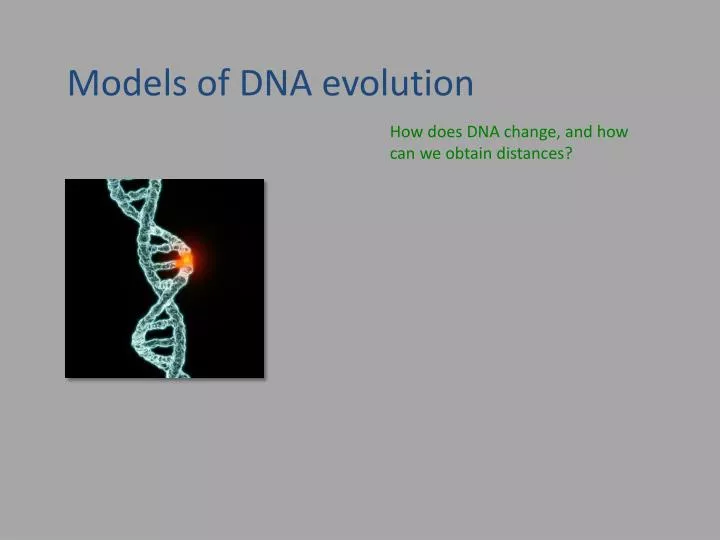
Models of DNA evolution. How does DNA change, and how can we obtain distances?. The Jukes-Cantor model. Thomas H. Jukes (1906-1999) King JL Jukes TH 1969. Non- DarwinianEvolution . Science 164: 788-798. Charles R. Cantor (°1942). The Jukes-Cantor model.

E N D
Models of DNA evolution How does DNA change, and how can we obtain distances?
The Jukes-Cantor model Thomas H. Jukes (1906-1999) King JL Jukes TH 1969. Non-DarwinianEvolution. Science 164: 788-798. Charles R. Cantor (°1942)
The Jukes-Cantor model in the JC model, each base in the sequence has an equal chance of changing, u, into one of the three other bases u A G u u u u T C u
The Jukes-Cantor model fictionalising, each base has a chance of (4/3)u of changing to a base randomly drawn from all 4 possibilities A G u/3 u/3 u/3 u/3 u/3 T C u/3
The Jukes-Cantor model the probability of no event is given by the zero term of a Poisson distribution e-m my PrY=y = y! 537 hits 576 squares average hit per square = 0.9323 probability of not being hit e-0.9323*0.93230 0! = = 0.3936 not at all expected number of squares hit 226.74
The Jukes-Cantor model e-m my PrY=y = y! 537 hits 576 squares average hit per square = 0.9323 probability being hit once e-0.9323*0.93231 1! = = 0.3670 not at all 1x expected number of squares hit 226.74 211.39
The Jukes-Cantor model e-m my PrY=y = y! 537 hits 576 squares average hit per square = 0.9323 probability of being hit twice e-0.9323*0.93232 2! = = 0.1711 not at all 1x 2x expected number of squares hit 226.74 211.39 98.54
The Jukes-Cantor model e-m my PrY=y = y! 537 hits 576 squares average hit per square = 0.9323 probability of being hit four times e-0.9323*0.93234 4! = = 0.012 not at all 1x 2x 3x 4x 5+ expected number of squares hit 226.74 211.39 98.54 30.62 7.131.6 observed number of squares hit 229 211 93 35 71
The Jukes-Cantor model e-m my PrY=y = y! A G u/3 probability of no event = e-(4/3)ut probability of ≥1 event = 1 - e-(4/3)ut u/3 probability of C at the end of a branch that started with A = (¼)(1 - e-(4/3)ut) u/3 u/3 u/3 probability that a site is different at two ends of a branch = (¾)(1 - e-(4/3)ut) T C u/3
The Jukes-Cantor model the expected difference per site between two sequences increases with branch length but reaches a plateau at 0.75 y = (¾)(1 - e-(4/3)ut)
The Jukes-Cantor model not using the J&C correction will distort the tree C B C B A D A D least squares tree the real tree expected uncorrected sequence differences
The Jukes-Cantor model the J&C model assumes no difference in substitution rates between transversions and transitions A G u/3 u/3 u/3 u/3 u/3 T C u/3
Kimura’s two-parameter model the Kimura model allows a difference in substitution rate between transversions and transitions A G a b b b b T C a a number of transitions R = = 2b number of transversions
Kimura’s two-parameter model - - t t Prob(transition|t) = ¼ - ½ e + ¼ e probability that a transition will occur in a time interval t 2R+1 2 R+1 R+1 a R = 2b
Kimura’s two-parameter model - - t t Prob(transition|t) = ¼ - ½ e + ¼ e probability that any tranversion will occur in a time interval t t Prob(transversion|t) = ½ - ½ e 2R+1 2 2 R+1 R+1 R+1
Kimura’s two-parameter model total (50% different) transitions transversions R=10
Kimura’s two-parameter model total (50% different) transversions transitions R=2
Tamura-Nei models the T&N models allow asymmetric base frequencies pA,G,C,T: relative proportion of A,G,C,T in the pool pR= pA+ pG pY = pC+ pT