Download
1 / 17
210 likes | 436 Views
Canny Edge Detector. However, usually there will still be noise in the array E[i, j], i.e., non-zero values that do not correspond to any edge in the original image. In most cases, these values will be smaller than those indicating actual edges.

E N D
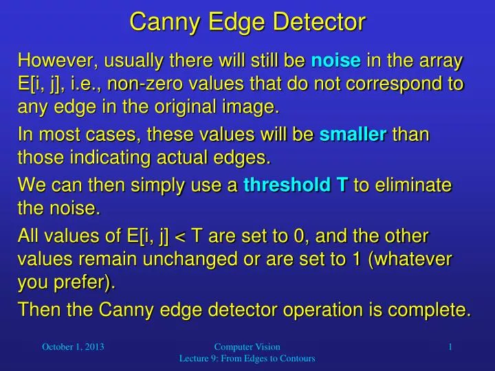
Canny Edge Detector • However, usually there will still be noise in the array E[i, j], i.e., non-zero values that do not correspond to any edge in the original image. • In most cases, these values will be smaller than those indicating actual edges. • We can then simply use a threshold T to eliminate the noise. • All values of E[i, j] < T are set to 0, and the other values remain unchanged or are set to 1 (whatever you prefer). • Then the Canny edge detector operation is complete. Computer Vision Lecture 9: From Edges to Contours
220 213 183 170 120 78 209 215 200 180 131 101 211 202 182 119 87 71 176 165 121 101 100 82 100 105 90 84 61 69 79 85 97 56 54 38 grayscale image intensity values of same image Canny Edge Detector - Example • Let us look at the following (already smoothed) sample image and perform Canny edge detection on it: Computer Vision Lecture 9: From Edges to Contours
-0.5 -22.5 -16.5 -49.5 -36 0 -4.5 9.5 13.5 10.5 -17 0 -1.5 -17.5 -41.5 -40.5 -23 0 5.5 -15.5 -39.5 -52.5 -37 0 -10 -32 -41.5 -16.5 -17 0 -36 -49 -39.5 -2.5 12 0 -3 -29.5 -13 -12 -5 0 -68 -45.5 -24 -28 -26 0 5.5 -1.5 -23.5 -12.5 -4 0 -20.5 -6.5 -10.5 -17.5 -19 0 0 0 0 0 0 0 0 0 0 0 0 0 Q[i, j] P[i, j] Canny Edge Detector - Example • Applying the vertical and horizontal gradient filters gives us the following results: Computer Vision Lecture 9: From Edges to Contours
4.5 24.4 21.3 50.6 39.8 0 186 293 309 282 295 0 5.7 23.4 57.3 66.3 43.6 0 345 228 226 218 212 0 37.4 58.5 57.3 16.7 20.8 0 196 213 226 261 305 0 68.1 54.2 27.3 30.5 26.5 0 183 213 208 203 191 0 21.2 6.7 25.7 21.5 19.4 0 165 193 246 216 192 0 0 0 0 0 0 0 0 0 0 0 0 0 M[i, j] [i, j] Canny Edge Detector - Example • Based on P[i, j] and Q[i, j], we can now compute the magnitude and orientation of the gradient: Computer Vision Lecture 9: From Edges to Contours
Remember the directions: 0 3 3 0 3 0 0 1 1 1 1 0 0 1 1 2 3 0 1 0 3 0 1 1 1 0 0 2 [i,j] 2 0 0 1 1 0 0 0 0 0 0 0 0 3 0 1 [i, j] Canny Edge Detector - Example • This allows us to compute the sector [i, j] for each angle [i, j]: Computer Vision Lecture 9: From Edges to Contours
0 24.4 0 50.6 0 0 0 0 0 1 0 0 0 0 57.3 66.3 0 0 0 0 1 1 0 0 0 58.5 57.3 0 0 0 0 1 1 0 0 0 68.1 54.2 0 0 26.5 0 1 1 0 0 0 0 0 0 0 0 0 0 0 0 0 0 0 0 0 0 0 0 0 0 0 0 0 0 0 0 E[i, j] final result Canny Edge Detector - Example • The last steps are nonmaxima suppression and thresholding (here we use T = 30): Computer Vision Lecture 9: From Edges to Contours
edge pixels edge locations in original image Canny Edge Detector - Example • Finally we visualize the detected edge pixels (0 = white, 1 = black) and indicate the precise edge locations (the pixels’ lower right corners) in the original image: Computer Vision Lecture 9: From Edges to Contours
Evaluating Edge Detector Performance • How can we decide which type of edge detector we should use in our application? • For this purpose, we need to find a method for evaluating the performance of these detectors. • First of all, we need to create one of more test images for which we know the actual locations and orientations of edges. • A straightforward idea is to just draw an image showing geometric objects. • One possible measure for edge detector performance is called the figure of merit. Computer Vision Lecture 9: From Edges to Contours
Evaluating Edge Detector Performance • The figure of merit FM is computed as follows: with number of detected edges IA, number of ideal edges II, distance between the actual and ideal edges (as matched by an appropriate algorithm) d, and constant for penalizing displaced edges . Computer Vision Lecture 9: From Edges to Contours
Evaluating Edge Detector Performance • The maximum value of FM is 1, which indicates perfect performance. • The closer FM is to 0, the poorer the performance. • Of course even a poor edge detector can perform very well in artificial images that show, for example, only perfect rectangles. • In order to perform a more meaningful analysis, we should add noise to our test images and see how well our edge detector can handle it. • One possibility is to simulate varying degrees of Gaussian noise in our test images. Computer Vision Lecture 9: From Edges to Contours
Probability for new intensity i’ of pixel probability original intensity i of pixel intensity Simulating Gaussian Noise • In order to simulate Gaussian noise, change the intensity of each pixel according to a Gaussian random distribution: standard deviation of Gaussian determines amount of noise Computer Vision Lecture 9: From Edges to Contours
probability intensity original intensity i of pixel new intensity i’ Simulating Gaussian Noise • To simulate a Gaussian random distribution, keep on choosing 2D random points in the marked rectangular area until one of them is under the Gaussian curve. • Set i’ to the horizontal coordinate of that point. Computer Vision Lecture 9: From Edges to Contours
1 strong (robust) edge detector figure of merit weak edge detector 0 0 50 100 of Gaussian noise Evaluating Edge Detector Performance • We can then measure the figure of merit as a function of the Gaussian noise added to the input image: Computer Vision Lecture 9: From Edges to Contours
From Edges to Contours • In order to represent a region boundary, we have to link its local edges. • Such a representation is called a contour. • Closed contours indicate region boundaries. • Open contours are usually parts of region boundaries with gaps due to noise or low contrast. • We can represent a contour as an ordered list of edges or as a curve. • A curve is a mathematical model of a contour. Computer Vision Lecture 9: From Edges to Contours
Edge Relaxation • The edge images generated by edge detection techniques (Sobel, Canny, etc.) are usually noisy. • In these images, contours may be visible to the human eye, but they may contain gaps, and there are isolated edges that do not belong to an actual contour. • We can use the edge relaxation technique to fill the gaps and remove the isolated edges. • It is an iterative method that assigns confidence values to edges and updates these values. Computer Vision Lecture 9: From Edges to Contours
f d a c i g h e b Edge Relaxation • Typically, this technique works on crack edges: pixel pixel pixel pixel pixel pixel Computer Vision Lecture 9: From Edges to Contours
Edge Relaxation • Edges h and i can be used for non-maxima suppression similar to the Canny detector. We will not discuss this here. • The edge pattern at an edge e can be described as a pair of integers: the number of connecting edges on the left (edges a, b, c) and the number of connecting edges on the right (d, f, g). • Since the left and right sides are exchangeable, we simply write the smaller number first, e.g. 0-1, 1-3, 2-2. • These edge patterns determine whether we should increase or decrease the current confidence value for e or leave it unchanged. Computer Vision Lecture 9: From Edges to Contours