Download
1 / 10
120 likes | 303 Views
Canny Edge Detector. The Skeleton of the Canny Edge Detector. Smooth the Image with Gaussian Filter Compute the Gr a dient Magnitude and Orientation using finite-difference approximations for the partial derivatives, Apply nonmaxima suppression to the gr a dient magnitude,

E N D
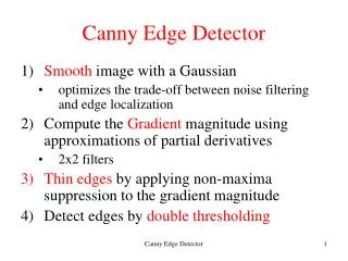
The Skeleton of the Canny Edge Detector • Smooth the Image with Gaussian Filter • Compute the Gradient Magnitude and Orientation using finite-difference approximations for the partial derivatives, • Apply nonmaxima suppression to the gradient magnitude, • Use the double thresholding algorithm to detect and link edges
Smoothing • Let I[i,j] denote the image and G[i,j,σ] be a Gaussian smoothing filter σ is the spread of the Gaussian and controls the degree of smoothing. • The result of convolution of I[i,j] with G[i,j,σ] gives an array of smoothed data as: s[i,j]= G[i,j,σ] * I[i,j]
Gradient Calculation • Firstly, the gradient of the smoothed array S[i,j] is used to produce the x and y partial derivatives • If the Sobel operator is used to obtain a 2-D spatial gradient,
Nonmaxima Suppression • Once the edge direction is known, the next step is to relate the edge direction to a direction that can be traced in an image. So if the pixels of a 5x5 image are aligned as follows: • x x x x xx x x x xx x a x xx x x x xx x x x x • Then, it can be seen by looking at pixel "a", there are only four possible directions when describing the surrounding pixels • 0 degrees (in the horizontal direction), • 45 degrees (along the positive diagonal), • 90 degrees (in the vertical direction), or • 135 degrees (along the negative diagonal).
Edge direction • Therefore, any edge direction falling within the yellow range (0 to 22.5 & 157.5 to 180 degrees) is set to 0 degrees. Any edge direction falling in the green range (22.5 to 67.5 degrees) is set to 45 degrees. Any edge direction falling in the blue range (67.5 to 112.5 degrees) is set to 90 degrees. And finally, any edge direction falling within the red range (112.5 to 157.5 degrees) is set to 135 degrees.
Nonmaximum suppression • Consider the four direction d1,d2,d3,d4 identified by the 0o,45o,90o,135o orientations • For each pixel (i,j): • Find the direction, dk, which best approximates the direction • If M[i,j] is smaller than at least one of its two neighbors along dk, assign I[i,j]=0; otherwise assign I[i,j]=M[i,j]
Hysteresis Thresholding • The image output by NONMAX- SUPPRESSION I[i,j] still contains the local maxima created by noise. How do we get rid of these? • If we set a low threshold in the attempt of capturing true but weak edges, some noisy maxima will be accepted too(false contours); • The values of true maxima along a connected contours may fluctuate above and below the threshold, fragmenting the result edge. • A solution is hysteresis thresholding
Hysteresis Thresholding • Two threshold values, TL and TH are applied to I[i,j]. Here TL < TH • For all the edge points in I[i,j], and scanning I[i,j] in a fixed order: 1. Locate the next unvisited edge pixel, I[i,j], such tht I[i,j]>TH; 2. Starting from I[i,j], follow the chains of connected local maxima, in both directions perpendicular to the edge normal, as long as I[i,j]>TL. Mark all visited points, and save a list of all locations of all points in the connected contour found. The output is a set of list, each describing the position of a connected contour in the image.