Download
1 / 45
450 likes | 509 Views
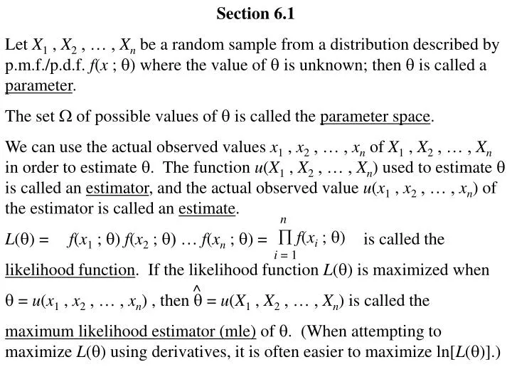
Section 6.1 Let X 1 , X 2 , … , X n be a random sample from a distribution described by p.m.f./p.d.f. f ( x ; ) where the value of is unknown; then is called a parameter . The set of possible values of is called the parameter space .

E N D
Section 6.1 Let X1 , X2 , … , Xn be a random sample from a distribution described by p.m.f./p.d.f. f(x ; ) where the value of is unknown; then is called a parameter. The set of possible values of is called the parameter space. We can use the actual observed values x1 , x2 , … , xn of X1 , X2 , … , Xn in order to estimate . The function u(X1 , X2 , … , Xn) used to estimate is called an estimator, and the actual observed value u(x1 , x2 , … , xn) of the estimator is called an estimate. L() = is called the likelihood function. If the likelihood function L() is maximized when = u(x1 , x2 , … , xn) , then = u(X1 , X2 , … , Xn)is called the maximum likelihood estimator (mle) of . (When attempting to maximize L() using derivatives, it is often easier to maximize ln[L()].) n f(xi ; ) i = 1 f(x1 ; ) f(x2 ; ) … f(xn ; ) = ^
The preceding discussion can be generalized in a natural way by replacing the parameter by two or more parameters (1 , 2 , …).
1. Consider each of the following examples (in the textbook). (a) Consider a random sample X1 , X2 , … , Xn from a Bernoulli distribution with success probability p. This sample will consist of 0s and 1s. What would be an “intuitively reasonable” formula for an estimate of p? n Xi i = 1 —— = X n Imagine that a penny is spun very fast on its side on a flat, hard surface. Let each Xi be 1 when the penny comes to rest with heads facing up, and 0 otherwise. Look at the derivation of the maximum likelihood estimator of p at the beginning of Section 6.1. n n xi i = 1 n xi i = 1 L(p) = p (1 p) for 0 p 1 n xi i = 1 n n xi i = 1 ln L(p) = ln p + ln(1 p)
n xi i = 1 n n xi i = 1 d [ln L(p)] ────── = dp ──── p ────── 1 p n xi i = 1 d [ln L(p)] ────── = 0 p = dp ──── = x n Notice that the second derivative is negative for all 0 < p < 1, which implies p = x does indeed maximize ln L(p). n xi i = 1 n n xi i = 1 d 2[ln L(p)] ────── = dp2 ──── p2 ────── (1 p)2 n Xi i = 1 —— = X n ^ is the maximum likelihood estimator of p. x is an estimate of p, and p =
(b) Consider a random sample X1 , X2 , … , Xn from a geometric distribution with success probability p. This sample will consist of positive integers. Decide if there is an “intuitively reasonable” formula for an estimate of p, and then look at the derivation of the maximum likelihood estimator of p in Text Example 6.1-2. Imagine that a penny is spun very fast on its side on a flat, hard surface. Let each Xi be the number of spins until the penny comes to rest with heads facing up. n Xi = i = 1 the total number of spins n = the total number of heads n —— = n Xi i = 1 1 — X n xi n i = 1 L(p) = pn (1 p) for 0 p 1 n xi n i = 1 ln L(p) = n ln p + ln(1 p)
n xi n i = 1 n ── p d [ln L(p)] ────── = dp ────── 1 p n 1 ──── = ─ x d [ln L(p)] ────── = 0 p = dp n xi i = 1 Notice that the second derivative is negative for all 0 < p < 1, which implies p = 1/ x does indeed maximize ln L(p). n xi n i = 1 d 2[ln L(p)] ────── = dp2 n ── p2 ────── (1 p)2 1 — X ^ n —— = n Xi i = 1 is the maximum likelihood estimator of p. 1/ x is an estimate of p, and p =
(c) Consider a random sample X1 , X2 , … , Xn from an exponential distribution with mean . This sample will consist of positive real numbers. Decide if there is an “intuitively reasonable” formula for an estimate of , and then look at the derivation of the maximum likelihood estimator of in Text Example 6.1-1. n Xi i = 1 —— = X n n xi i = 1 ──── exp ──────── for 0 n L() = n xi i = 1 ──── n ln() ln L() = n xi i = 1 ──── 2 d [ln L()] ────── = d n ──
n xi i = 1 —— = x n d [ln L(p)] ────── = 0 = d n 2 xi i = 1 ──── + 3 d 2[ln L(p)] ────── = d 2 n ── 2 n xi i = 1 —— n n3 ——— n xi i = 1 Substituting = into the second derivative results in 2 n xi i = 1 —— n which is negative, implying = does indeed maximize ln L(). n Xi i = 1 —— = X n ^ is the maximum likelihood estimator of . x is an estimate of , and =
2. (a) Consider the situation described immediately following Text Example 6.1-4. Suppose X1 , X2 , … , Xn is a random sample from a gamma(,1) distribution. Note how difficult it is to obtain the maximum likelihood estimator of . Then, find the method of moments estimator of . n xi i = 1 1 n xi i = 1 exp ──────────────── for 0 [()] n L() = n xi i = 1 n xi i = 1 ln L() = n ln () ( 1) ln When this derivative is set equal to 0, it is not possible to solve for , since there is no easy formula for /() or (). n xi i = 1 n /() ──── () d [ln L()] ────── = d ln
The preceding discussion can be generalized in a natural way by replacing the parameter by two or more parameters (1 , 2 , …). ~ A method of moments estimator of a parameter is one obtained by setting moments of the distribution from which a sample is taken equal to the corresponding moments of the sample, that is, When the number of equations is equal to the number of unknowns, the unique solution is the method of moments estimator. n (Xi / n) , i = 1 n (Xi2 / n) , i = 1 n (Xi3 / n) , etc. i = 1 E(X) = E(X 2) = E(X 3) = If E[u(X1 , X2 , … , Xn)] = , then the statistic u(X1 , X2 , … , Xn) is called an unbiased estimator of ; otherwise, the estimator is said to be biased. (Text Definition 6.1-1)
2. (a) Consider the situation described immediately following Text Example 6.1-4. Suppose X1 , X2 , … , Xn is a random sample from a gamma(,1) distribution. Note how difficult it is to obtain the maximum likelihood estimator of . Then, find the method of moments estimator of . n (Xi / n) i = 1 n (Xi / n) i = 1 E(X) = (1) = = n Xi i = 1 —— = X n ~ is the method of moments estimator of . =
(b) Suppose X1 , X2 , … , Xn is a random sample from a gamma(,3) distribution. Again, note how difficult it is to obtain the maximum likelihood estimator of . Then, find the method of moments estimator of . n xi i = 1 ──── 3 n xi i = 1 1 exp ──────────────── for 0 [() 3] n L() = n xi i = 1 ──── 3 n xi i = 1 ln L() = ( 1) ln n ln () n ln3 n xi i = 1 n /() ──── () d [ln L()] ────── = d n ln3 ln When this derivative is set equal to 0, it is not possible to solve for , since there is no easy formula for /() or ().
(b) Suppose X1 , X2 , … , Xn is a random sample from a gamma(,3) distribution. Again, note how difficult it is to obtain the maximum likelihood estimator of . Then, find the method of moments estimator of . n Xi i = 1 —— 3n n (Xi / n) i = 1 n (Xi / n) i = 1 E(X) = (3) = 3 = = n Xi i = 1 —— = 3n X — 3 ~ is the method of moments estimator of . =
3. Study Text Example 6.1-5, find the maximum likelihood estimator, and compare the maximum likelihood estimator with the method of moments estimator. n xi for 0 i = 1 1 L() = n n xi i = 1 ln L() = n ln + ( 1) ln n xi i = 1 d [ln L()] ────── = d n ── + ln n ———— = n ——— n lnxi i = 1 d [ln L(p)] ────── = 0 = d n xi i = 1 ln
n ———— = n ——— n lnxi i = 1 d [ln L(p)] ────── = 0 = d n xi i = 1 ln Notice that the second derivative is negative for all 0 , which implies = does indeed maximize ln L(). d 2[ln L(p)] ────── = d 2 n ── 2 n ——— n lnxi i = 1 ^ n ——— n lnXi i = 1 = is the maximum likelihood estimator of , which is not equal to the method of moments estimator of derived in Text Example 6.1-5.
4. (a) A random sample X1 , X2 , … , Xn is taken from a N( , 2) distribution. The following are concerned with the estimation of one of, or both of, the parameters in the N( , 2) distribution Study Text Example 6.1-3, and note that in order to verify that the solution point truly maximizes the likelihood function, we must verify that 2 2(ln L) ——— 12 2(ln L) ——— 22 2(ln L) ——— 12 – > 0 at the solution point 2(ln L) ——— 12 and that < 0 at the solution point. – n —— 2 2(lnL) ——— = 22 n 1 n — – — (xi – 1)2 222 23i=1 2(lnL) ——— = 12 2(lnL) ——— = 12 –1 n — (xi – 1) 22i=1
1 n — (xi – x)2 ni = 1 When 1 = x and 2 = , then – n2 ———— n (xi – x)2 i=1 –n3 ————— n 2 (xi – x)2 i=1 2(lnL) ——— = 12 2(lnL) ——— = 22 2(lnL) ——— = 12 0 2 2 n5 ————— > 0 n 2 (xi – x)2 i=1 2(lnL) ——— 12 2(lnL) ——— – 22 2(lnL) ——— = 12 We see then that 3 – n2 ———— < 0 . n (xi – x)2 i=1 2(lnL) ——— = 12 and that (b) Study Text Example 6.1-6.
The preceding discussion can be generalized in a natural way by replacing the parameter by two or more parameters (1 , 2 , …). ~ A method of moments estimator of a parameter is one obtained by setting moments of the distribution from which a sample is taken equal to the corresponding moments of the sample, that is, When the number of equations is equal to the number of unknowns, the unique solution is the method of moments estimator. n (Xi / n) , i = 1 n (Xi2 / n) , i = 1 n (Xi3 / n) , etc. i = 1 E(X) = E(X 2) = E(X 3) = If E[u(X1 , X2 , … , Xn)] = , then the statistic u(X1 , X2 , … , Xn) is called an unbiased estimator of ; otherwise, the estimator is said to be biased. (Text Definition 6.1-1)
4.-continued (c) (d) Study Text Example 6.1-4. Do Text Exercise 6.1-2. n 1 (xi– )2 ——— exp – ——— = i=1 (2)1/2 2 L() = n – (xi – )2 i=1 1 ——— exp ————— (2)n/2 2 n 1 n – — ln(2) – — (xi – )2 2 2 i=1 ln L() = n 1 n – — + — (xi – )2 2 22i=1 d(lnL) ——— = d = 0
n 1 n – — + — (xi – )2 2 22i=1 d(lnL) ——— = d = 0 1 n — (xi – )2 ni=1 d2(lnL) ——— = d2 n 1 n — – — (xi – )2 22 3i=1 = 1 n — (xi – )2 ni=1 –n3 ————— n 2 (xi – )2 i=1 d2(lnL) ——— = d2 < 0 When = , then 2 which implies that L has been maximized. 1 n — (Xi – )2 ni=1 ^ = is the mle (maximum likelihood estimator) of = 2. (Now look at Corollary 5.4-3.) 1 n — (Xi – )2 = ni=1 2n (Xi – )2 — E ———— = ni=1 2 ^ E() = E
1 n — (Xi – )2 = ni=1 2n (Xi – )2 — E ———— = ni=1 2 2 — n = 2 n ^ E() = E ^ 1 n — (Xi – )2 ni=1 Consequently, = is an unbiased estimator of = 2.
4.-continued (e) Return to Text Exercise 6.1-2, and find the maximum likelihood estimator of = ; then decide whether or not this estimator is unbiased. n 1 (xi– )2 ——— exp – ——— = i=1 (2)1/2 22 L() = n – (xi – )2 i=1 1 ——— exp ————— (2)n/2n 22 n 1 n – — ln(2) – n ln – — (xi – )2 2 22i=1 ln L() = n 1 n – — + — (xi – )2 3i=1 d(lnL) ——— = d = 0
1/2 1 n — (xi – )2 ni=1 d2(lnL) ——— = d2 n 3 n — – — (xi – )2 2 4i=1 = 1/2 1 n — (xi – )2 ni=1 – 2n2 ———— n (xi – )2 i=1 d2(lnL) ——— = d2 < 0 When = , then which implies that L has been maximized. 1/2 1 n — (Xi – )2 ni=1 ^ = is the mle (maximum likelihood estimator) of = . Recall from part (d): 1 n — (Xi – )2 ni=1 ^ = is the mle (maximum likelihood estimator) of = 2.
1/2 1 n — (Xi – )2 ni=1 ^ = is the mle (maximum likelihood estimator) of = . We now want to know whether or not this estimator is unbiased. Recall from part (d): 1 n — (Xi – )2 ni=1 ^ = is the mle (maximum likelihood estimator) of = 2. We proved that this estimator is unbiased. It can be shown that the mle of a function of a parameter is that same function of the mle of . However, as we have just seen, the expected value of a function is not generally equal to that function of the expected value.
1/2 1/2 1 n — (Xi – )2 = ni=1 n (Xi – )2 — E ———— = ni=1 2 ^ E() = E ??? We need to find the expected value of the square root of a random variable having a chi-square distribution Suppose random variable U has a 2(r) distribution. Then, using a technique similar to that used in Text Exercises 5.2-3 and 5.5-17, we can show that ([r+1]/2) E(U1/2) = 2———— (r/2) (and you will do this as part of Text Exercise 6.1-14).
1/2 ([r+1]/2) E(U1/2) = 2———— (r/2) n (Xi – )2 — E ———— = ni=1 2 ^ E() = ([n+1]/2) — 2———— = n (n/2) 2 ([n+1]/2) —————— n (n/2) 1/2 1 n — (Xi – )2 ni=1 ^ = is a biased estimator of = . n (n/2) —————— 2 ([n+1]/2) ^ An unbiased estimator of = is = 1/2 (n/2) —————— 2 ([n+1]/2) n (Xi – )2 i=1 (This is similar to what you need to do as part of Text Exercise 6.1-14).
5. (a) Suppose X1 , X2 , … , Xn is a random sample from any distribution with finite mean and finite variance 2. If the distribution from which the random sample is taken is a normal distribution, then from Corollary 5.5-1 we know that X has a N( , 2/n) distribution This implies that X is an unbiased estimator of and has variance 2/n ; show that this is still true even when the distribution from which the random sample is taken is not a normal distribution. No matter what distribution the random sample is taken from, Theorem 5.3-3 tells us that since n Xi i = 1 n (1/n)Xi , then i = 1 X = = —— n n (1/n) = i = 1 n (1/n)22 = i = 1 E(X) = , and Var(X) = n(1/n)22 = 2/n The Central Limit Theorem tells us that when n is sufficiently large, the distribution of X is approximately a normal distribution.
(b) If the distribution from which the random sample is taken is a normal distribution, then from Text Example 6.1-4 we know that S2 is an unbiased estimator of 2. In Text Exercise 6.1-13, you will show that S2 is an unbiased estimator of 2even when the distribution from which the random sample is taken is not a normal distribution. Show that Var(S2) depends on the distribution from which the random sample is taken. 2 n Xi i = 1 2 n Xi2– i = 1 Var(S2) = E[(S2– 2)2] = E ——— n – 2 n– 1 We see that Var(S2) will depend on E(Xi), E(Xi2), E(Xi3), and E(Xi4). We know that E(Xi) = and E(Xi2) = no matter what type of distribution the random sample is taken from, but 2 + 2 E(Xi3) and E(Xi4) will depend on the type of distribution the random sample is taken from. If the random sample is taken from a normal distribution, Var(S2) =
If the random sample is taken from a normal distribution, Var(S2) = 1 n —— (Xi – X)2 = n– 1i =1 4n (Xi–X)2 ——— Var ———— = (n– 1)2i=1 2 Var (Now look at Theorem 5.5-2.) 4 ——— (2)(n 1) = (n– 1)2 24 —— n 1
6. (a) (b) Let X1 , X2 be a random sample of size n = 2 from a gamma( ,1) distribution (i.e., > 0). Show that X and S2 are each an unbiased estimator of . 2 First, we recall that E(X) = and E(S2) = for a random sample taken from any distribution with mean and variance 2 . Next, we observe that for a gamma(, ) distribution, = and 2 = . 2 Consequently, with = 1, we have E(X) = E(S2) = so that X and S2 are each , an unbiased estimator of . Decide which of X and S2 is the better unbiased estimator of . When we are faced with choosing between two (or more) unbiased estimators, we generally prefer the estimator with the variance. smaller Recall that Var(X) = 2 / n = / n = / 2 .
To find Var(S2), we observe (as done in Class Exercise 5.5-3(a)) that (X1– X)2 + (X2 – X)2 ———————— = 2 – 1 S2 = 2 2 X1 + X2X1 + X2 X1– ——— + X2 – ——— = 2 2 2 2 2 X1–X2X2–X1 ——— + ——— = 2 2 X1–X2 ——— = 2 X12– 2X1X2 +X22 ——————— 2 2 2 X12– 2X1 X2 +X22 ——————— – ( )2 = 2 Var(S2) = E[(S2)2] – [E(S2)]2 = E
6.-continued 2 X12– 2X1X2 +X22 ——————— – 2 = 2 Var(S2) = E[(S2)2] – [E(S2)]2 = E X14+ 4X12X22 +X24 – 4X13X2 + 2X12X22 – 4X1X23 ——————————————————— – 2 = 4 E 2E(X 4) + 6E(X 2)E(X 2) – 8E(X 3)E(X) – 42 ————————————————— = 4 2M////(0) + 6[M//(0)]2 – 8M///(0) – 42 ———————————————— 4
1 ——— (1 – t) ——— (1 – t)+1 ( + 1) ———— (1 – t)+2 M/(t) = M//(t) = M(t) = ( + 1)( + 2) ——————— (1 – t)+3 ( + 1)( + 2)( + 3) ————————— (1 – t)+4 M///(t) = M////(t) = M//(0) = ( + 1) M///(0) = ( + 1)( + 2) M////(0) = ( + 1)( + 2)( + 3)
6.-continued 2M////(0) + 6[M//(0)]2 – 8M///(0) – 42 ———————————————— = 4 Var(S2) = 2( + 1)( + 2)( + 3)+ 62( + 1)2 – 82( + 1)( + 2) – 42 —————————————————————————— = 4 6( + 1)( + 2)+ 62( + 1)2 – 62( + 1)( + 2) – 42 ———————————————————————— = 4 6( + 1)( + 2) – 62( + 1) – 42 ——————————————— = 4 12( + 1) – 42 ——————— = 4 82+ 12 ———— = 4 22+ 3 > / 2 = Var(X) Consequently, the better unbiased estimator of is X . (Note that the same type of approach used here would be needed to prove the result in part (d) of Text Exercise 6.1-4.)
7. (a) Let X1 , X2 , … , Xn be random sample from a U(0 , ) distribution. Find the expected value of X ; then find a constant c so that W1 = cX is an unbiased estimator of . First, we recall that E(X) = for a random sample taken from any distribution with mean and variance 2 . Next, we observe that for a U(0, ) distribution, = and 2 = . /2 2/12 Consequently, we have E(X) = /2 , and E(cX) = , if we let c = . 2 Therefore, W1 = is 2X an unbiased estimator of .
(b) Find the expected value of Yn = max(X1 , X2 , … , Xn), which is the largest order statistic; then find a constant c so that W2 = cYn is an unbiased estimator of . Since Yn is the largest order statistic, and its p.d.f. is gn(y) = n [F(y)]n–1f(y) for 0 < y < where f(x) and F(x) are respectively the p.d.f and d.f. for the distribution from the random sample is taken. 0 if x 0 1 — for 0 < x < f(x) = F(x) = x / if 0 < x 1 if < x E(Yn) = y n [F(y)]n–1f(y) dy = y n [y / ]n–1 [1 / ]dy = 0 0
nyn —dy = n nyn+1 ——— = (n+1)n n —— n + 1 0 y = 0 n+ 1 —— n We have E(cYn) = , if we let c = . n+ 1 —— Yn n Therefore, W2 = is an unbiased estimator of .
7.-continued (c) Decide which of W1 orW2 is the better unbiased estimator of . When we are faced with choosing between two (or more) unbiased estimators, we generally prefer the estimator with the variance. smaller Var(W1) = Var(2X) = 4Var(X) = 42 / n = 4(2 / 12) / n = 2 / (3n) . 2 n+ 1 —— Yn n n+ 1 —— n Var(W2) = Var = Var(Yn) = 2 n+ 1 —— n {E(Yn2) – [E(Yn)]2} = This we need to find out. This we already know.
nyn+2 ——— = (n+2)n n —— 2 n + 2 nyn+1 —dy = n E(Yn2) = y2 n [y / ]n–1 [1 / ]dy = 0 0 y = 0 2 2 2 n+ 1 —— n n+ 1 —— n n —— 2 n + 2 n – —— n + 1 Var(W2) = {E(Yn2) – [E(Yn)]2} = 2 — = Var(W1) 3n (n+ 1)2 = ———— – 1 2 = n(n + 2) 1 ——— 2 n(n + 2) Consequently, the better unbiased estimator of is W2 .
7.-continued (d) Explain why Ynis the mle of . n f(xi;) = i=1 1 — n 1 — for 0 < x < L() = f(x) = Since > 0, the value for which maximizes L() is the smallest possible positive value for . must be no smaller than each of the observed values x1 , x2 , …, xn ; otherwise L() = 0. Consequently, L() is maximized when = max(x1 , x2 , …, xn). It follows that the mle of must be the largest order statistic Yn = max(X1 , X2 , …, Xn) .
8. (a) Let X represent a random variable having the U(– 1/2 , + 1/2) distribution from which the random sample X1 , X2 , X3 is taken, and let Y1 < Y2 < Y3 be the order statistics for the random sample. We consider the statistics W1 = X = (the sample mean), W2 = Y2 (the sample median), W3 = (the sample midrange). X1+X2 + X3 ————— 3 Y1+Y3 ——— 2 Text Exercise 8.3-14 is closely related to this Exercise. Find E(W1) and Var(W1). For a U( – 1/2 , + 1/2) distribution, we have = b+ a —— = 2 + 1/2 + – 1/2 ——————— = 2
For a U( – 1/2 , + 1/2) distribution, we have = 2 = b+ a —— = 2 + 1/2 + – 1/2 ——————— = 2 (b– a)2 ——— = 12 ( + 1/2 – [ – 1/2])2 ———————— = 12 1 — 12 Consequently, E(W1) = E(X) = and Var(W1) = Var(X) = 1 —– = 12n 1 — 36
8.-continued (b) Find E(W2) and Var(W2). (This can be done easily by using Class Exercise #8.3-4(b).) b+ a —— = 2 + 1/2 + – 1/2 ——————— = 2 E(W2) = E(Y2) = ( + 1/2 – [– 1/2])2 ———–————— = 20 1 — 20 (b – a)2 ———– = 20 Var(W2) = Var(Y2) =
8.-continued (c) Find E(W3) and Var(W3). (This can be done easily by using Class Exercise #8.3-4(b).) b+ 3a ——— + 4 3b+ a ——— 4 Y1 + Y3 E(W3) = E ——— = 2 E(Y1) + E(Y3) —————— = 2 ———————— = 2 b+ a —— = 2 + 1/2 + – 1/2 ——————— = 2 1 — Var(Y1 + Y3) = 4 Y1 + Y3 Var(W3) = Var ——— = 2 Var(Y1) + Var(Y3) + 2Cov(Y1, Y3) —————————————— = 4
Var(Y1) + Var(Y3) + 2Cov(Y1, Y3) —————————————— = 4 Var(Y1) + Var(Y3) + 2[E(Y1Y3) – E(Y1)E(Y3)] —————————————————— = 4 3(b – a)2 ———– + 80 3(b – a)2 ———– + 2 80 [b – a]2 ——— + ab – 5 b+ 3a ——— 4 3b+ a ——— 4 —————————————————————————— = 4 3 — + 80 3 — + 2 80 1 1 — + 2 – — – 5 4 (4 – 1)(4 + 1) ——————— 16 —————————————————————— = 4 1 — 40 (d) (e) Why is each of W1 , W2 , and W3 an unbiased estimator of ? We have seen that E(W1) = E(W2) = E(W3) = . Decide which of W1 , W2 , and W3 is the best estimator of ? W3 is the best estimator, since it has the smallest variance.