Magnitudes and moment Source time function Source spectra Stress drop

1. Source parameters I • Magnitudes and moment • Source time function • Source spectra • Stress drop • Earthquake scaling and statistics • Fault scaling and statistics • Asperities and barriers Richter in his living room

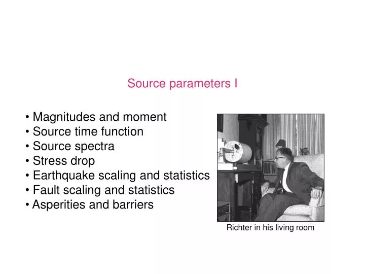
2. Source parameters I: Magnitudes and moment log(a) event1 event2 event3 distance Richter noticed that the vertical offset between every two curves of maximum displacement is independent of the distance. Thus, one can measure the magnitude of a given event with respect to the magnitude of a reference event as: where A and A0 are the largest amplitudes of the event and the reference event, respectively, and  is the epicentral distance.

3. Source parameters I: Magnitudes and moment The actual data Richter was using is this:

4. Source parameters I: Magnitudes and moment From a table of values of A0, an approximate empirical formula has been derived for the logarithm of the reference event, and the local magnitude is defined as: This definition is only valid for Southern California and only when the Wood-Anderson seismograph is being used.

5. Source parameters I: Magnitudes and moment • Richter arbitrarily chose a magnitude 0 event to be an earthquake that would show a maximum combined horizontal displacement of 1 micrometer on a seismogram recorded using a Wood-Anderson torsion seismometer 100 km from the earthquake epicenter. • Problems with Richter’s magnitude scale: • The Wood-Anderson seismograph is no longer in use, and cannot record magnitudes greater than 6.8. • Local scale for South California, and therefore difficult to compare with other regions. • Nevertheless, Local Magnitudes are still reported sometimes because many building have resonant frequencies near 1Hz, close to that of the Wood-Anderson (0.8 Hz), so ML can serve as an indication of the structural damage an earthquake can cause.

6. Source parameters I: Magnitudes and moment • Several other magnitude scales have been defined, but the most commonly used are: • Surface-wave magnitude (MS). • Body-wave magnitude (mb). • Moment magnitude (Mw).

7. Source parameters I: Magnitudes and moment • Both surface-wave and body-waves magnitudes are a function of the ratio between the displacement amplitude, A, and the dominant period, T, and are given by: • where the distance correction accounts for the decrease of A with distance due to geometrical spreading and attenuation. • mb is calculated from the early portion of the body wave train, usually the P wave. Common US practice is to use the first 5 S of the record, and period of less than 3 S, usually 1 S on instruments with peak response near 1 S. • Ms is measured either using the largest amplitude (zero to peak) of the surface waves, or using the amplitude of the Rayleigh waves at 20 S, which often have the largest amplitude. • Magnitude scales are logarithmic, so an increase in one unit indicates a ten-fold increase in the displacement.

8. Source parameters I: Magnitudes and moment • Main limitations: • Totally empirical and as such have no physical meaning (note that the expression inside the logarithm has physical units of mm/S). • Magnitude estimates vary noticeably with azimuth due to amplitude radiation pattern - although this difficulty is partially reduced by averaging. • Body and surface wave magnitudes do not correctly reflect the size of large earthquakes.

9. Source parameters I: Magnitudes and moment • The moment magnitude is a function of the seismic moment, M0, as follows: • where M0 is in dyne-cm. The seismic moment is a physical quantity (as opposed to earthquake magnitude) that measures the strength of an earthquake. It is equal to: where: G is the shear modulus A = LxW is the rupture area D is the average co-seismic slip (It may be calculated from the amplitude spectra of the seismic waves.)

10. Source parameters I: Magnitudes and moment Note that an increase of one magnitude unit corresponds to a 101.5 ≈ 32 times increase in the amount of energy released: where m1 and m2 are two moment magnitudes. The pasta-quake analogy:

11. Source parameters I: Magnitudes and moment • Note that: • mb saturates above 6 • MS saturates above 8

12. Source parameters I: Magnitudes and moment Just so that you don’t get the false impression that earthquake slip distribution is smooth and everywhere close to the average slip

13. Source parameters I: Magnitudes and moment Magnitude classification (from the USGS): 0.0-3.0 : micro 3.0-3.9 : minor 4.0-4.9 : light 5.0-5.9 : moderate 6.0-6.9 : strong 7.0-7.9 : major 8.0 and greater : great

14. Source parameters I: Magnitudes and moment Richter TNT for Seismic Example Magnitude Energy Yield (approximate) -1.5 6 ounces Breaking a rock on a lab table 1.0 30 pounds Large Blast at a Construction Site 1.5 320 pounds 2.0 1 ton Large Quarry or Mine Blast 2.5 4.6 tons 3.0 29 tons 3.5 73 tons 4.0 1,000 tons Small Nuclear Weapon 4.5 5,100 tons Average Tornado (total energy) 5.0 32,000 tons 5.5 80,000 tons Little Skull Mtn., NV Quake, 1992 6.0 1 million tons Double Spring Flat, NV Quake, 1994 6.5 5 million tons Northridge, CA Quake, 1994 7.0 32 million tons Hyogo-Ken Nanbu, Japan Quake, 1995; Largest Thermonuclear Weapon 7.5 160 million tons Landers, CA Quake, 1992 8.0 1 billion tons San Francisco, CA Quake, 1906 8.5 5 billion tons Anchorage, AK Quake, 1964 9.0 32 billion tons Chilean Quake, 1960 10.0 1 trillion tons (San-Andreas type fault circling Earth) 12.0 160 trillion tons (Fault Earth in half through center, OR Earth's daily receipt of solar energy)

15. Source parameters I: Magnitudes and moment

16. Source parameters I: Source time function Moment magnitude has become the standard measure of earthquake size, but it requires more analysis and understanding of the seismic signal.

17. Source parameters I: Source time function

18. Source parameters I: Source time function Imagine the source time function resulting from a point source radiating an impulse moving at velocity VR along a line of length L that is embedded within a medium whose seismic velocity is V. The signal’s duration is:

19. Source parameters I: Source time function For points far from the fault, i.e. r>>L: Thus, the time pulse becomes: It follows that the maximum duration occurs at 180 degrees of the rupture propagation direction, whereas the minimum duration occurs at the rupture direction.

20. Source parameters I: Source time function The Haskell fault model: But slip at a given point does not occur instantaneously. The slip history is often modeled as a ramp function. The source time function depends on the time derivative of the slip history. A ramp time history has a derivative of a boxcar. When convolved with the boxcar time function due to rupture propagation, a trapezoidal time function results, whose width is equal to the rupture and rise times.

21. Source parameters I: Source time function The duration of the radiated pulse varies with azimuth. The area of the pulse is the same at all azimuths, and therefore the amplitude of the source time function is inversely proportional to the duration. This effect is known as the directivity effect. In some cases the directivity effect helps to identify rupture plane, since no similar effect is associated with the auxiliary plane.

22. Source parameters I: Source time function The ratio between the time pulse (the width of the boxcar) and the predominant period of the seismic wave is: If this ratio is small, the source is “seen” as a point source, whereas if this ratio is large, there are finite source effects.

23. Source parameters I: Source spectra How would this source time function look in the frequency domain? According to the Haskell fault model the source time function results from the convolution of two boxcar time functions. The transform of a boxcar of height 1/T and length T is:

24. Source parameters I: Source spectra Thus, the spectral amplitude of the source signal is the product of the seismic moment of two sinc terms: where TR and TD are the rupture and rise times, respectively. Often, amplitude spectra are plotted using a logarithm scale. Taking the logarithm of the above gives:

25. Source parameters I: Source spectra It is useful to approximate sinc(x) as 1 for x<1 and as 1/x for x>1. This approach yields: Note the two corner frequencies dividing the into 3 parts.

26. Source parameters I: Source spectra While in principle, by studying the spectra of real earthquakes, we can recover M0, TR and TD, in practice things are more complicated than that.

27. Source parameters I: Source spectra As rupture lengths increase, the seismic moments, rise times and rupture durations increase. Thus, the corner frequencies move to the left, i.e. to lower frequencies.

28. Source parameters I: Source spectra • Ms is measured at periods of 20S, and it saturates beyond M0>10^25 dyn-cm. • mb is measured at periods of 1S, and it saturates beyond M0>10^22 dyn-cm. • Similar saturation effects occur for other magnitude scales which are measured at specific frequencies.

29. Source parameters I: Source spectra Again, this is how the moment magnitude is defined: where M0 is in dyne-cm. In contrast to body and surface wave magnitudes, the moment magnitude does not saturate.

30. Source parameters I: Stress drop One approach to find L is to analyze the amplitude of the spectrum, identify the corner frequency, and use that to assess the rupture duration. The latter divided by an average rupture speed of 0.7-0.8 of the shear wave speed gives L.

31. Source parameters I: Stress drop • What emerges from this is that co-seismic stress drop is constant over a wide range of sizes. • The constancy of the stress drop implies linear scaling between co-seismic slip and rupture length. slope=3 Figure from: Hanks, 1977

32. Source parameters I: The scaling of fault length and slip Normalized slip profiles of normal faults of different length. Normalized displacement From Dawers et al., 1993

33. Source parameters I: The scaling of fault length and slip Displacement versus fault length What emerges from this data set is a linear scaling between displacement and fault length. Figure from: Schlische et al, 1996

34. Source parameters I: The Gutenberg-Richter statistics Fortunately, there are many more small quakes than large ones. The figure below shows the frequency of earthquakes as a function of their magnitude for a world-wide catalog during the year of 1995. This distribution may be fitted with: where n is the number of earthquakes whose magnitude is greater than M. This result is known as the Gutenberg-Richter relation. Figure from simscience.org

35. Source parameters I: The Gutenberg-Richter statistics • While the a-value is a measure of earthquake productivity, the b-value is indicative of the ratio between large and small quakes. Both a and b are, therefore, important parameters in hazard analysis. Usually b is close to a unity. • Note that the G-R relation describes a power-law distribution.

36. Source parameters I: The Gutenberg-Richter distribution versus characteristic distribution G-R distribution characteristic distribution • Two end-member models can explain the G-R statistics: • Each fault exhibits its own G-R distribution of earthquakes. • There is a power-law distribution of fault lengths, with each fault exhibiting a characteristic distribution.

37. Source parameters I: Fault distribution and earthquake statistics Cumulative length distribution of subfaults of the San Andreas fault. Scholz, 1998

38. Source parameters I: Fault distribution and earthquake statistics Loma Prieta

39. Source parameters I: Fault distribution and earthquake statistics • In conclusion: • For a statistically meaningful population of faults, the distribution is often consistent with the G-R relation. • For a single fault, on the other hand, the size distribution is often characteristic. • Note that the extrapolation of the b-value inferred for small earthquakes may result in under-estimation of the actual hazard, if earthquake size-distribution is characteristic rather than power-law. Question: what gives rise to the drop-off in the small magnitude with respect to the G-R distribution?

40. Source parameters I: The controls on rupture final dimensions Seismological observations show that: Co-seismic slip is very heterogeneous. Slip duration (rise time) at any given point is much shorter than the total rupture duration Example from the 2004 Northern Sumatra giant earthquake Preliminary result by Yagi. Uploaded from: www.ineter.gob.ni/geofisica/tsunami/com/20041226-indonesia/rupture.htm

41. Source parameters I: The controls on rupture final dimensions • Barriers are areas of little slip in a single earthquake (Das and Aki, 1977). • Asperities are areas of large slip during a single earthquake (Kanamori and Stewart, 1978). The origin and behavior with time of barriers and asperities: Fault geometry - fixed in time and space? Stress heterogeneities - variable in time and space? Both?

42. Source parameters I: The controls on rupture final dimensions According to the barrier model (Aki, 1984) maximum slip scales with barrier interval. If this was true, fault maps could be used to predict maximum earthquake magnitude in a given region.

43. Source parameters I: The controls on rupture final dimensions But quite often barriers fail to stop the rupture… The 1992 Mw7.3 Landers (CA): The 2002 Mw7.9 Denali (Alaska): Figure from: pubs.usgs.gov Figure from: www.cisn.org

44. Source parameters I: The controls on rupture final dimensions While in the barrier model ruptures stop on barriers and the bigger the rupture gets the bigger the barrier that is needed in order for it to stop, according to the asperity model (Kanamori and Steawart, 1978) earthquakes nucleate on asperities and big ruptures are those that nucleate on strong big asperities. That many ruptures nucleate far from areas of maximum slip is somewhat inconsistent with the asperity model. Further reading: • Scholz, C. H., The mechanics of earthquakes and faulting, New-York: Cambridge Univ. Press., 439 p., 1990. • Aki, K., Asperities, barriers and characteristics of earthquakes, J. Geophys. Res., 89, 5867-5872, 1994.