Download
1 / 43
430 likes | 628 Views
Nonlinear Data Assimilation using an extremely efficient Particle Filter. Peter Jan van Leeuwen Data-Assimilation Research Centre University of Reading. The Agulhas System. In-situ observations. In-situ observations. In situ observations Transport through Mozambique Channel.

E N D
Nonlinear Data Assimilation using an extremely efficient Particle Filter Peter Jan van Leeuwen Data-Assimilation Research Centre University of Reading
Data assimilation Uncertainty points to use of probability density functions. P(u) 0.0 0.5 1.0 u (m/s)
Data assimilation: general formulation Bayes theorem: Solution is pdf! NO INVERSION !!!
How is this used today? • Present-day data-assimilation systems are based on linearizations and search for one optimal state: • (Ensemble) Kalman filter: assumes Gaussian pdf’s • 4DVar: smoother assumes Gaussian pdf for initial state and observations (no model errors) • Representer method: as 4DVar but with Gaussian model errors • Combinations of these
Prediction: smoothers vs. filters • The smoother solves for the mode of the conditional joint pdf p( x0:T | d0:T) (modal trajectory). • The filter solves for the mode of the conditional marginal pdf p( xT | d0:T). For linear dynamics these give the same prediction.
Filters maximize the marginal pdf • Smoothers maximize the joint pdf These are not the same for nonlinear problems !!!
Example Nonlinear model 2 xn xn+1 = 0.5 xn + _________ + nn 1 + e (xn - 7) Initial pdf x0 ~ N(-0.1, 10) Model noise nn ~ N(0, 10)
Example: marginal pdf’s Note: mode is at x= - 0.1 Note: mode is at x=8.5 x0 xn
Example: joint pdf Mode joint pdf x0 xn Modes marginal pdf’s
And what about the linearizations? • Kalman-like filters solve for the wrong state: gives rise to bias. • Variational methods use gradient methods, which can end up in local minima. • 4DVar assumes perfect model: gives rise to bias.
Where do we want to go? • Represent pdf by an ensemble of model states • Fully nonlinear Time
How do we get there? Particle filter? Use ensemble with the weights.
What are these weights? • The weight w_i is the pdf of the observations given the model state i. • For M independent Gaussian distributed observation errors:
Particle Filter degeneracy: resampling • With each new set of observations the old weights are multiplied with the new weights. • Very soon only one particle has all the weight… • Solution: Resampling: duplicate high-weight particles are abandon low-weight particles
Problems • Probability space in large-dimensional systems is ‘empty’: the curse of dimensionality u(x1) u(x2) T(x3)
Standard Particle filter Not very efficient !
Specifics of Bayes Theorem I We know from Bayes Theorem: Now use : in which we introduced the transition density
Specifics of Bayes Theorem II This can be rewritten as: q is the proposal transition density, which might be conditioned on the new observations! This leads finally to:
Specifics of Bayes Theorem III How do we use this? A particle representation of Giving: Now we choose from the proposal transition density for each particle i.
Particle filter with proposal density Stochastic model Proposed stochastic model: Leads to particle filter with weights
Meaning of the transition densities = the probability of this specific value for the random model error. For Gaussian model errors we find: A similar expression is found for the proposal transition
Experiment: Lorentz 1963 model (3 variables x,y,z, highly nonlinear) x-value Measure only X-variable y-value
Standard Particle filter with resampling20 particles Typically 500 particles needed ! X-value Time
Particle filter with proposal transition density 3 particles X-value Time
Particle filter with proposal transition density 3 particles Y-value (not observed) Time
However: degeneracy • For large-scale problems with lots of observations this method is still degenerate: • Only a few particles get high weights; the other weights are negligibly small. • However, we can enforce almost equal weight for all particles:
Equal weights • Write down expression for each weight with q deterministic: Prior transition density Likelihood 2. When H is linear this is a quadratic function in for each particle. 3. Determine the target weight:
Almost Equal weights I 1 4 3 Target weight 2 5 4. Determine corresponding model states, e.g. solving alpha in
Almost equal weights II • But proposal density cannot be deterministic: • Add small random term to model equations from a pdf with broad wings e.g. Gauchy • Calculate the new weights, and resample if necessary
Application: Lorenz 1995 N=40 F=8 dt = 0.005 T = 1000 dt Observe every other grid point Typically 10,000 particles needed
Ensemble evolution at x=2020 particles Time step
Isn’t nudging enough? Only nudged Nudged and weighted
Isn’t nudging enough? Unobserved variable Only nudged Nudged and weighted
Conclusions The nonlinearity of our problem is growing • Particle filters with proposal transition density: • solve for fully nonlinear solution • very flexible, much freedom • application to large-scale problems straightforward
Future • Fully nonlinear filtering (smoothing) forces us to concentrate on the transition densities, so on the errors in the model equations. • What is the sensitivity to our choice of the proposal? • What can we learn from studying the statistics of the ‘nudging’ terms? • How do we use the pdf???