Download
1 / 28
280 likes | 289 Views
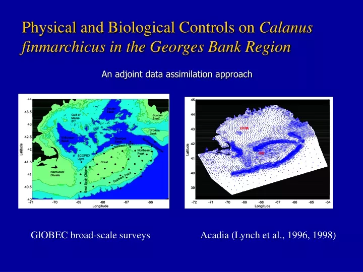
Physical and Biological Controls on Calanus finmarchicus in the Georges Bank Region. An adjoint data assimilation approach. GlOBEC broad-scale surveys. Acadia (Lynch et al., 1996, 1998). Climatological C. f. distributions (GLOBEC , 1995-1999). Jan: abundances are low (C3<C2)<C5

E N D
Physicaland Biological Controls on Calanus finmarchicus in the Georges Bank Region An adjoint data assimilation approach GlOBEC broad-scale surveys Acadia (Lynch et al., 1996, 1998)
Climatological C. f. distributions (GLOBEC , 1995-1999) Jan: abundances are low (C3<C2)<C5 Feb: reproduction starts; C2>C3>C4>c5; centers are advected along the bank Mar-Apr: abundances are high May: C2,C3 abundances decline Jun: abundances drop sharply on the crest; high centers retain near the Southern Flank (C2, C3) and along the periphery of the bank (C4,C5); C5>C4>>C3>C2 Data courtesy of Durbin et al.
Questions • Where are the off-bank sources in late winter? • How are the off-bank sources imported to the bank to initiate the growing season? • How do the biological processes & physical transports result in the observed C. f. distributions? • How do these animals disappear from the crest of the bank?
Campbell et al., 2001 Molting Flux F2 F3 F4 C2 C3 C4 C5 R2 Molting from C1 and C2 mortality R5 R3 R4 Mortality (R<0) C5 molting, mortality, diapause emergence/entry
Forward Model: Infer R_i and C_i (t=0) by minimizing: First guess: R_i=0, C_i(t=0)=(Cobs on the bank; 0 off-bank)
Observations Model results
Abundance Inferred Source/sinks Molting flux advection
Inferred biological terms Important Source regions: the GB, the Georges Basin, Wilkinson Basin, the Browns banks (Feb-Apr.) Mortality: Mar-April, Southern Flank (Food limitation, Campbell et. al., 2001); May-Jun crest (predation, Bollens et al., 1999 )
Inferred C3 controls Net bio-gain/loss Advection: loss: Wilkinson, Georges Basins; Gains: northwest crest, Georges Basin and the south tip of GSC. Bio-gain: Feb-Apri ; Bio-loss: June; Feb-Apri: Bio>Adv June decline: Bio-losses; Jan-Feb Feb-Mar Mar-Apr Apr-May May-June
Inferred C5 controls Net bio-gain/loss Jan-Feb: Advective convergence (Northern Flank,Georges Basin) Feb-Apr: Bio, Adv both are important Bio>Adv June: Bio~Adv Jan-Feb Feb-Mar Apr-May Mar-Apr May-June
Conclusions 1. The Scotian Shelf, GOM are important sources of C4 and C5 in late winter. The convergence of advective C5 flux near the northern periphery of the bank seems to be important to seed the bank. 2. Both biological reactions and physical advection are important for the observed distributions. Physical transports increase from winter to spring.
Conclusions 3. Biological gains are major contributors for high abundances in Spring; Biological losses are mainly responsible for the decline of C2-C4 in June, while for C5, both biological loss and advective transport are responsible for the June decline; 4. Molting fluxes largely exceed mortality rates (C2-C3, Jan.-Jun.). 5. Mar.15-Apr.15, mortality is high near the southern Flank; May.15-Jun.15, mortality is high on the crest. 6. Results are inferred from modeled flow fields and data on the GB only. More accurate inference about the controls in the off-bank region needs data in those areas and improved estimate of circulation.
Future Work • Incorporate more data: N3—C1(pump data)—C2—Adult stages; data in other regions. • Use 3D model to study vertical migration as well as the controls already included. • Explore the connection between interannual, synoptic (e.g., storm driven) physical variability & biological variability. • Sensitivity study to rank the physical & biological controls • Extend the study area to a larger scale (e.g., North Atlantic).
Molting Flux (F) C: Concentration; D: stage duration; T: temperature; CF: Food concentration Campbell et al., 2001
C2 stage duration T limited T & Chl limited Chla: OReilly & Zetlin (1996); T (Lynch et al., 1996)
Procedure • Choose a best first guess of control vector U. • Integrate the forward model and calculate the cost function. • Run the adjoint model to calculate the gradient of J to U. • Use a descent algorithm to find a new value of U. • Repeat from the second step until a satisfactory solution has been achieved.
unconstrained constrained The inversion reduces model-data misfit by ~90%
Computed tendencies Increasing season: Jan-Apr; Decline season: Apr-Jun; Centers are located along the bank periphery with advective signatures.
Inferred C2 controls Jan-Feb: biological gains first appears near the Northern edge of the Bank. Feb-May Biological gains/loses and advective transport are important June: bio.-lose is mainly responsible for the decline
Inferred C4 controls Net bio-gain/loss High abundances in spring: bio-gains; June-decline: bio-losses. Jan-Feb Feb-Mar Apr-May Mar-Apr May-June
Hypotheses • Georges Bank populations limited by C. f. supply from GOM diapause stock during winter. • GB dynamics influenced by growth conditions on the bank during spring (food limited in April). • GOM sources to GB become more and more important during spring and summer. Courtesy of http://globec.whoi.edu, phase1 projects
MARMAP Observations(1977-1987) Courtesy of www.at-sea.org
Figure 4. Estimates of predation impact by 5 predators, based on feeding rates and abundances of predators and prey from Broad Scale Survey samples. Impact is expressed as percent of the stocks of Calanus and Pseudocalanus removed daily, assuming that the predators are non-selective (E=0), and consume these species in the same proportions as they occur. Prey of Clytia are nauplii, prey of the other predators are copepodites and adults (Bollens et. al., online.sfsu.edu).