Download

1 / 37
380 likes | 571 Views
Motion. Optical flow. Measurement of motion at every pixel. Problem definition: optical flow. Key assumptions color constancy : a point in H looks the same in I For grayscale images, this is brightness constancy small motion : points do not move very far

E N D
Optical flow Measurement of motion at every pixel
Problem definition: optical flow • Key assumptions • color constancy: a point in H looks the same in I • For grayscale images, this is brightness constancy • small motion: points do not move very far • This is called the optical flow problem • How to estimate pixel motion from image H to image I? • Solve pixel correspondence problem • given a pixel in H, look for nearby pixels of the same color in I
Lukas-Kanade flow Solution: solve least squares problem • minimum least squares solution given by solution (in d) of: • The summations are over all pixels in the K x K window • This technique was first proposed by Lukas & Kanade (1981) • described in Trucco & Verri reading • Prob: we have more equations than unknowns
Iterative Refinement • Iterative Lukas-Kanade Algorithm • Estimate velocity at each pixel by solving Lucas-Kanade equations • Warp H towards I using the estimated flow field • - use image warping techniques • Repeat until convergence
Coarse-to-fine optical flow estimation u=1.25 pixels u=2.5 pixels u=5 pixels u=10 pixels image H image H image I image I Gaussian pyramid of image H Gaussian pyramid of image I
Coarse-to-fine optical flow estimation warp & upsample run iterative L-K . . . image J image H image I image I Gaussian pyramid of image H Gaussian pyramid of image I run iterative L-K
Multi-resolution Lucas Kanade Algorithm • Compute Iterative LK at highest level • For Each Level i • Take flow u(i-1), v(i-1) from level i-1 • Upsample the flow to create u*(i), v*(i) matrices of twice resolution for level i. • Multiply u*(i), v*(i) by 2 • Compute It from a block displaced by u*(i), v*(i) • Apply LK to get u’(i), v’(i) (the correctionin flow) • Add corrections u’(i), v’(i) to obtain the flow u(i), v(i) at ith level, i.e., u(i)=u*(i)+u’(i), v(i)=v*(i)+v’(i)
Optical flow competition • http://vision.middlebury.edu/flow/eval/
Global Flow • Dominant Motion in the image • Motion of all points in the scene • Motion of most of the points in the scene • A Component of motion of all points in the scene • Global Motion is caused by • Motion of sensor (Ego Motion) • Motion of a rigid scene • Estimation of Global Motion can be used to • Video Mosaics • Image Alignment (Registration) • Removing Camera Jitter • Tracking (By neglecting camera motion) • Video Segmentation etc.
Global Flow Application: Image Alignment
Global Flow • Special Case of General Optical Flow Problem • Can be solved by using Lucas Kanade algorithm. • Specialized algorithms exist that perform better by further constraining the problem.
Motion Models • First we look for a parametric form of global flow vector. Global Flow occurs because of 3D rigid motion of either the sensor or the scene. 3D Rigid Motion (If is small) Also neglecting the higher order terms
Iterative Refinement • Iterative Algorithm • Estimate global flow by solving linear system Aa=B • Warp H towards I using the estimated flow • - use image warping techniques (to be covered later) • Repeat until convergence or a fixed number of iterations
Coarse-to-fine global flow estimation u=1.25 pixels u=2.5 pixels u=5 pixels u=10 pixels image H image H image I image I Gaussian pyramid of image H Gaussian pyramid of image I
Coarse-to-fine global flow estimation warp & upsample Compute Flow Iteratively . . . image J image H image I image I Gaussian pyramid of image H Gaussian pyramid of image I Compute Flow Iteratively
Basic Components • Pyramid Construction • Motion Estimation • Image Warping • Coarse to Fine Refinement
Result of Global Motion Estimation Image ‘t’ Image ‘t+1’ Affine Model output 4 Pyramids Level 5 Iterations/Pyramid Level
Unwarp Mosaic • http://research.microsoft.com/en-us/um/cambridge/projects/visionimagevideoediting/unwrap/
Summary • Things to take away from this lecture • Optical flow problem definition • Aperture problem and how it arises • Assumptions • Brightness constancy, small motion, smoothness • Derivation of optical flow constraint equation • Lukas-Kanadeequation • Conditions for solvability • meanings of eigenvalues and eigenvectors • Iterative refinement • Newton’s method • Coarse-to-fine flow estimation • Applications • Image alignment / Video mosaic